If the fibers added to the structure are curved fibers, a Curl tab appears in the right panel. Curved fibers can bend in four modes, selectable in the Curl Mode pull-down menu: Spiral, Sine, Random and Curvature. The curl parameters are different for these modes. The default mode is Random.
Spiral
Spiral curved fibers form a three-dimensional curve that winds around an axis. The spirals are defined by the Spiral Diameter and the Spiral Shift. The spiral shift is the distance between the same relative positions in two consecutive loops of the spiral. The segment lengths for spiral fibers are optimized to obtain smoothly curved fibers for the chosen parameters.
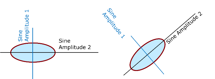
The Sine Length controls the length of one periodic sine section. A sine curvature can only be applied if the amplitude is set to positive values. Then, the fibers oscillate in direction of the main axis.
Sine Amplitude 1 and Sine Amplitude 2 describe the oscillation amplitude in the direction of the main axis. This is shown below for an elliptical fiber.
Sine fibers have only one sinusoidal component when the Sine Amplitude 1 (or Sine Amplitude 2) is 0, while the other sine amplitude is set to a positive value. Sine fibers with a combination of components are obtained when both sine amplitudes are set to positive values. For example, with the following values:
Initially, keep the default values of Sine Length 1, and Sine Length 2, whereasthe Sine Amplitude 1 and Sine Amplitude 2 are set to 0, as is the Torsion Start Angle. These parameters produce straight fibers.
When the same fibers are created with a smaller Sine Length 2 (75 µm) and a Sine Amplitude 2 of 10 µm, the sine fibers appear curved.
When these same curved sine fibers are created with a Torsion Start Angle that follows a uniform distribution in the interval 0 to 90º, the sine fibers appear curved and twisted.
Random
Curved Random fibers consist of straight fiber segments of a given Segment Length. Its value determines the length of the linear parts that build the fiber. This way small values lead to well resolved fibers with smooth curving. A large segment length leads to fibers with long straight segments.
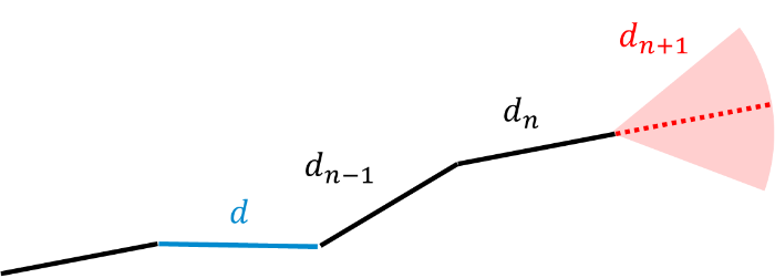
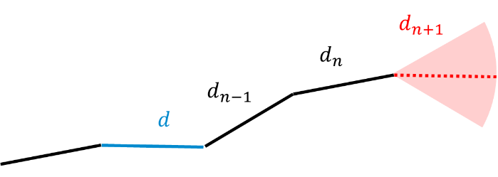
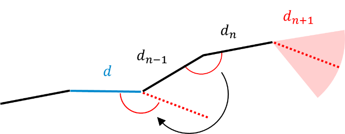
The first segment is placed in space according to the Center and Orientation values defined under the Fiber tab. The curved fiber follows a main fiber direction given by the fiber orientation. The first segment is the middle segment. The other segments are attached to both ends according to the Straightness and Randomness parameters.
The checking or un-checking of Isotropic controls the direction in which the parameters Local Straightness, Global Straightness,and Randomness are applied to the new segment. These parameter values (between 0 and 1) define the direction of each newly attached segment and determine how strongly a fiber may change direction from one segment to the next.
Randomness corresponds to the standard deviation of the Gaussian distribution with mean value 0. The direction of the new segment is determined by the following rule:
(9) Random Curved Fibers
where
: main direction of the fiber (orientation applied on first segment),
: direction of the current segment,
: direction of the last segment,
: Local Straightness
: Global Straightness
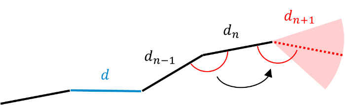
For the shape of the fiber, there are four main cases considering the parameters for local and global straightness ( and ). The impact of these parameters on each new segment is explained below.
The blue segment is the center segment which is the first segment placed according to the parameters for orientation () and center defined in the Fiber tab. The red dotted line would be the new segment for , as the Randomness value controls the width of the red area.
The previous direction is kept, i.e. the fiber tends to be locally straight.
(10)
The main fiber direction is kept, i.e. the fiber tends to be globally straight.
(11)
The previous curvature is kept.
(12)
The angle between the current and the last segment, defined by the previous curvature, is considered for the attachment of the new segment. This angle is applied between the direction of the new segment and the main direction, i.e. the fiber always bends with respect to the main direction. Thus, it tends to be globally straight, while the local curvature is taken into account.
In the following examples, all parameters are left unchanged while curved circular fibers with a length of 100 µm are given varying Segment Length, as indicated.
The Curl Parameters are Isotropic by default. Alternatively, anisotropic curl parameters can be defined. This is done by unchecking Isotropic and entering the parameters for each direction (X, Y and Z) separately.
Here, the same curl parameter values are entered for the X- and Y-directions, whereas no deformation is allowed in Z-direction, where Local Straightness and Global Straightness have been set to 1 and Randomness to 0.
In this example, observe how the deformation of curved circular fibers occurs only in the XY-plane of an anisotropic-oriented structure (Anisotropy 1 =100 and Anisotropy 2 =1) when entering the anisotropic curl parameters shown above.
With values of Anisotropy 1 and Anisotropy 2 being 100 and 1, the generated fibers are oriented perpendicular to the Z-axis.
Views from the X- and the Y-direction show that there is no deformation of fibers in Z-direction. This is a consequence of setting the Randomness in Z-direction to zero.
The view from the Z-direction shows that the fibers are curved in the X and Y directions.
The Straightness values can be set between 0 and 1. The higher the value for Global Straightness,the more the fiber tends towards the main direction.
With a non-zero Global Straightness value, the fibers tend to return to the initial prescribed Orientation.
With a Global Straightness value of 1, the fibers globally keep the Orientation, while a Local Straightness of 0 leads to fibers locally keeping curvature.
The higher the value for Local Straightness the smoother the curves, as the local directions tend to be kept. If the Global Straightness value is 0, the fibers are not restrained to stay in the predefined Orientation.
A non-zero value of Local Straightness results in a reduction of the fibers’ curvature (compared to the structure with Local Straightness of 0 above).
A Local Straightness value of 1 leads to low curvature and straighter fibers.
A higher Global Straightness value, with a Local Straightness value of 1, results in almost straight fibers keeping the main direction.
Observe the effect of varying Local Straightness, Global Straightness and Randomness on a structure made of highly anisotropic (oriented in the Z-axis, Anisotropy 1 = 0.001, Anisotropy 2 = 1) curved circular fibers. All other parameters remain unchanged.
With Randomness set to zero, all segments have the same direction, resulting in straight fibers.
With a slightly higher Randomness value (0.01), curvature is introduced. With Global Straightness and Local Straightness set to 0, the predefined orientation is only applied to the initial segment and the curvature differs not much between adjacent segments, leading to spiral-like curves.
The fiber curvature increases with the Randomness value.
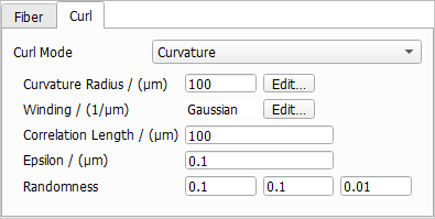
Curvature
The Curvature is only selectable for curved circular, curved hollow, curved rosetta, and curved angular fibers.
The Curvature Radius controls the radius of the spiral followed by the fiber. Choosing the values of Randomness and Winding to be 0 leads to loops with the radius defined by Curvature Radius.
The Correlation Length defines the length of the fiber section for which Curvature Radius and Winding are applied. For each of those sections, these parameters are applied anew. If none of the two parameters is set to a random distribution, the Correlation Length has no impact.
In the example below, the Curvature Radius is deviated uniformly between 10 and 50. The winding is set to the constant value 0.1. With a Correlation Length of 50 each spiral is different but with a Correlation Length of 100 the spirals with small radius are repeated. As the Winding is kept constant, the Correlation Length is only applied to the Curvature Radius.
For curvature the Epsilon determines the maximal difference of the discretized fiber from an analytical circle with the curvature of the fiber in the segment defined by the other parameters.
For each new segment a curvature is drawn corresponding to the curvature radius.
The correlation length determines when a new curvature is drawn. Within this correlation length the curvatures (and the winding) are interpolated to gain a smooth transition.
The curvature radius determines the direction of the new segment within the local 2D plane. The winding is the deviation from this plane for each segment.
If winding and curvature differ due to parameter distributions or randomness, the segment length is also not constant. It varies corresponding to the parameters applied to it.
The curvature radius drawn for the new segment defines an analytical circle. The value entered for epsilon then is the distance between the circle boundary and the new segment.
In the figure below, a new segment is applied (red) for two different epsilon values.
For constant parameters, 0 winding and 0 randomness all segments would lay within the same circle leading to an analytical circle.
The higher the Randomness value, the stronger are the changes of curvature radius and winding in each section. Setting Randomness = 0 creates loops and spirals.