The default stopping criterion of the LIR solver, Error Bound, uses the result of previous iterations, and predicts the final solution based on linear and quadratic extrapolation. The solver stops if the relative difference between computed and predicted solution is smaller than the specified error bound. The stopping criterion recognizes oscillations in the convergence behavior and prevents premature stopping at local minima or maxima. A damped convergence curve is fit through the oscillating curve and the solver stops then regarding the damped convergence curve.

If the Krylov method (under LIR - Advanced Options) is activated, the definition of Error Bound is somewhat different. Here, no prediction is made, instead the continuity between neighboring cells and the conservation of mass is checked. The maximal value is normalized by the mean flow and if this value is smaller than the Error Bound the simulation stops.

The Tolerance stopping criterion, the default stopping criterion for EJ, looks for stagnation of the method when the process becomes stationary, i.e. the improvement in the diffusivity value becomes extremely small from iteration to iteration.

In each iteration, the solver checks for the current computed value against the values of the last 100 iterations if there are any changes.

The computation is stopped if the maximal relative change is smaller than the value entered for Tolerance. When there is doubt about the quality of the solution, decrease the Tolerance value by a factor of ten. The drawback of this criterion is that the solver sometimes might stop too early in case of slow convergence rate or at local extrema of oscillatory convergence curves.

Control how many threads are used for the computation. Parallelization is possible if your license and hardware allow it.

The Parallelization Options dialog opens when clicking the Edit button and you can choose between Sequential, Parallel (Shared Memory), or Automatic Maximum of Threads.

Selecting Sequential will not apply parallelization and only one thread is used for the computation.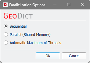

When Parallel (Shared Memory) is selected, the Number of Threads can be entered. Below, the Number of CPU Cores that the current machine has, the maximum number of Licensed Threads and the number of those licensed threads that are available (Available Threads) are shown in the dialog. Of course, the maximal number of parallel processes you can use, is the smallest of those three numbers.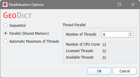

If Automatic Maximum of Threads is selected, the number of parallel processes is automatically selected for optimal speed, based on the CPU cores and licensed parallel processes.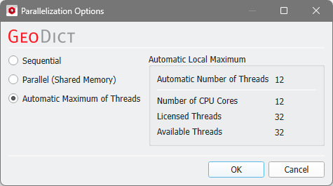

The Automatic Local Maximum of processes is automatically selected, which is the minimum of Number of CPU Cores, Licensed Threads, and Available Threads.

The LIR solver uses a very memory efficient adaptive grid structure for the simulations.

If the option Write Compressed Volume Fields is checked, then the adaptive grid is used as compression method for writing out *.hht files. This option allows to save 80-90% space on hard drive. The runtime for writing *.hht files is also reduced significantly. But the runtime for loading and uncompressing of compressed *.hht is increased by the amount of runtime that was saved for writing out compressed *.hht files.

If the option Write Compressed Volume Fields is not checked, then a usual regular grid is used for writing out *.hht files.

The Multigrid Method (see e.g. Wesseling, 2004) was introduced to speed-up the computation and reduce the runtime significantly. The main idea of Multigrid is the usage of multiple coarser adaptive grids to speed up convergence behavior but requires only little more memory.

The method is available to solve the Stokes and Stokes–Brinkman equations as well as for solving mechanics, diffusion, thermal, and electrical conduction and is enabled by default.

Another speed-up option to accelerate the convergence behavior of the LIR solver is called Krylov Subspace Method.

The runtime of the LIR solver depends on many different properties of the structure and the simulation parameters. The BiCGStab algorithm is used, which can reduce the runtime for challenging simulation very drastically.

Unfortunately, the Krylov method is not always faster than a simulation without the Krylov method and therefore we introduced an Automatic mode which uses some heuristics to choose the most efficient method based on structure, material parameters, and boundary conditions automatically. Of course, it is possible to explicitly enable (Enabled) or disable (Disabled) the method.

Depending on the material parameters and geometry of the structure, the underlying mathematical problem can vary in complexity, thus influencing the behavior of the solver. The more complex the problem is, the more stable the solver settings should be.

With the Relaxation number, the solver is adjusted from Stable (which results in higher number of iterations, slower time stepping, and longer solver run times), to Fast, which makes the solver run less iterations but implies the risk that the solver does not converge. The Relaxation is a parameter of the SOR method and must be between 0 and 2 to ensure convergence. For relaxation values smaller than one (<1.0), the simulation is more stable. For relaxation values larger than one (>1.0), the simulation converges faster.

The LIR solver can Optimize for Speed or Memory.

• If Speed is chosen, the solver constructs additional optimization structures. The runtime is decreased by up to 30% but requires up to 50% more memory compared to the other option.
• If Memory is chosen, the runtime is increased by up to 40% but the solver requires up to 50% less memory.

The Grid Type decides what kind of tree structure is used for the simulation.

The default option is LIR-Tree and should always be used. The solver uses an adaptive grid structure called LIR-tree and needs up to 10 times less runtime and memory compared to the Regular Grid option.

The solver can analyze the result field during the computation and improves the adaptive grid in places where more accuracy is needed. The LIR solver splits cells where a high gradient occurs.

The other Grid Options are fixed and shown for your reference only.