Uniaxial Experiment
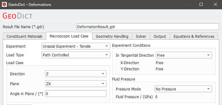
In an Uniaxial Experiment, the load is applied in one given direction. This direction can be either given by one of the coordinate directions (X, Y, Z), a given angle to one of the coordinate directions in each coordinate plane (e.g., XZ or YZ), or a shear experiment can be defined.
The available load types are Tensile, Compression or Shear. The choice of Tensile or Compression only affects the sign of the loads, for example negative tension equals compression. The load can be time-dependent, e.g., cyclic.
 Load Case
The choices available for the Load Case vary depending on whether Tensile, Compression or Shear is selected. For Tensile and Compression experiments, a direction, a Plane, and an Angle in Plane must be defined. For Shear experiments, the Shear Load must be selected. If Without Geometric Nonlinearity under the Geometry Handling tab is chosen, three different shear loads are available: Here, the theory of small deformations applies, therefore the Shear in XY direction corresponds to the shear in YX direction. Thus, three different shear options are available in this case: XY, XZ and YZ.
When the theory of small deformations does not apply (With Geometric Nonlinearity), there are three different cases for shear in X and Y directions: Shear in XY direction, shear in YX direction (the deformation gradient is asymmetric in those cases) and symmetric shear in X and Y directions (this is a superposition of the two other cases, the deformation gradient is symmetric in this case). Thus, nine different shear options are available for the geometric nonlinear case.
Refer to the Geometry Handling section for more information about the geometry options.
|
Experiment Conditions
The load conditions in the directions tangential to the load direction can be Free (zero mean stress/nominal stress in the geometry), Confined (zero mean strain/displacement gradient in the geometry) or Mixed. Free means that the structure can expand or contract freely to the load direction, whereas there is no expansion/contraction for confined boundary conditions. With Mixed tangential boundary conditions, two different conditions (Free or Confined) can be selected for the two tangential directions.
|
Fluid Pressure
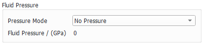
When the structure for the simulation contains pores, a fluid pressure model can be selected. With No Pressure, no pressure is applied (this is the default case).
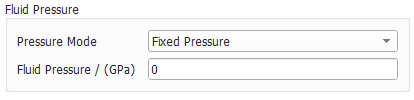
With Fixed Pressure, a fixed pressure can be given. This fixed pressure is applied at the start of the ElastoDict computations.
With the third option, Pressure Per Step, the applied pressure can be defined for each simulation step. These pressure steps must be entered in the Load Table (see further explanation below).
The pressure is always applied to all fluids in the structure. This means that it is not only applied to pores in the material, but also to the fluid which surrounds the structure.
|
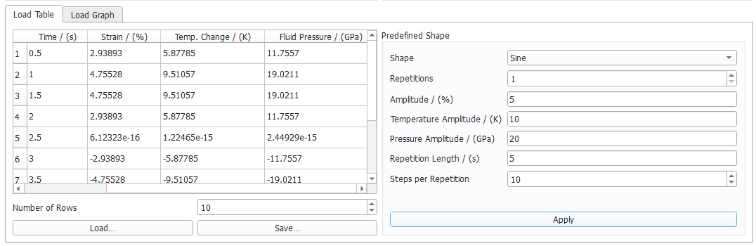
Load Definition (Load Table and Predefined Shape)
The load steps to be computed need to be specified in the Load Table, where a plot of the load curve can be seen under the Load Graph subtab. It is also possible to use a load curve of Predefined Shape like Linear, Sawtooth, or Sine, by selecting it from the pull-down menu on the right and clicking Apply, to set it in the Load Table and visualize it under Load Graph.
For the shapes Linear and Sine there is also the option to define the thermal conditions by setting the Temperature Change / (K) for the Linear shape and Temperature Amplitude / (K) for the Sine shape
In case Pressure Mode → Pressure Per Step is chosen, additionally to the load and temperature curve, the fluid pressure curve can be defined in Predefined Shape by setting the Pressure Change / (GPa) for the Linear shape or Pressure Amplidute / (GPa) for the Sine shape.
The load table can be loaded from and saved to a *.txt file with the Load… and Save… buttons.
Alternatively, the data from the load table can be entered from other software like Microsoft Excel® via copy and paste.
The time information from the load table is only used if the materials in the structure have a time-dependent behavior. When working with UMATs, this time information is passed to the UMAT.
|
Complex Load Experiment
The Complex Load Experiment allows to define more elaborate load scenarios, e.g., a tensile experiment followed by a shear load or multiple load directions at the same time. The load directions can be defined freely as a combination of normal and shear loads. The complete mean stress (nominal stress) or strain (displacement gradient) tensor for the geometry can be defined.
In this way, combinations of multiple loads directions are possible (e.g., biaxial load, triaxial load…). The load directions can be defined freely as a combination of normal and shear loads. In the screenshot below, a tensile strain of 2% in X-direction, a shear load of 1% in XY-direction and a tensile strain of 5% in Z-direction is set.
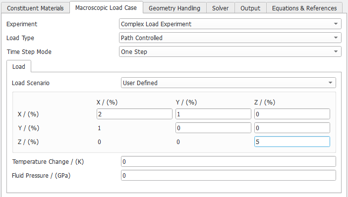
Possible options for Time Step Mode are One Step or Time Series.
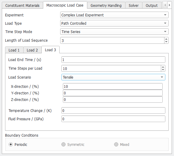
Whereas One Step consists of a single load step, a Time Series may consist of several load steps (Length of Load Sequence: 1, 2, 3…), where each load step (Load 1, Load 2, Load 3… tabs) is defined by a Load End Time, number of Time Steps per Load and a Load Scenario. The Load Scenario can be Tensile, Compression, Shear or User Defined.
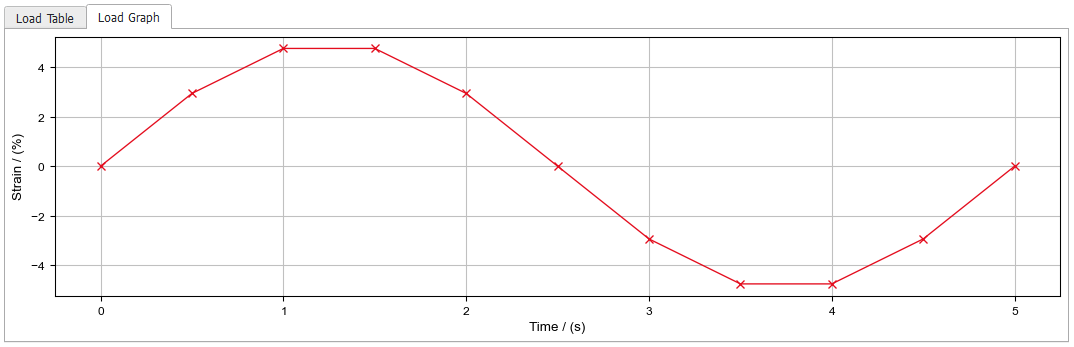
The total time of the load is the difference of the current Load End Time and the previous Load End Time; therefore, the load end time must be strictly increasing. Each load is divided in a given number of Time Steps per Load. The concept is illustrated in the following figure:
The load sequences can be combined as desired. You can e.g. do a compression in X-direction followed by a compression in Y-direction and a shear load.
In the example below, the 3rd load is subdivided into 10 time steps (Time Steps per Load) and the load scenario is Tensile.