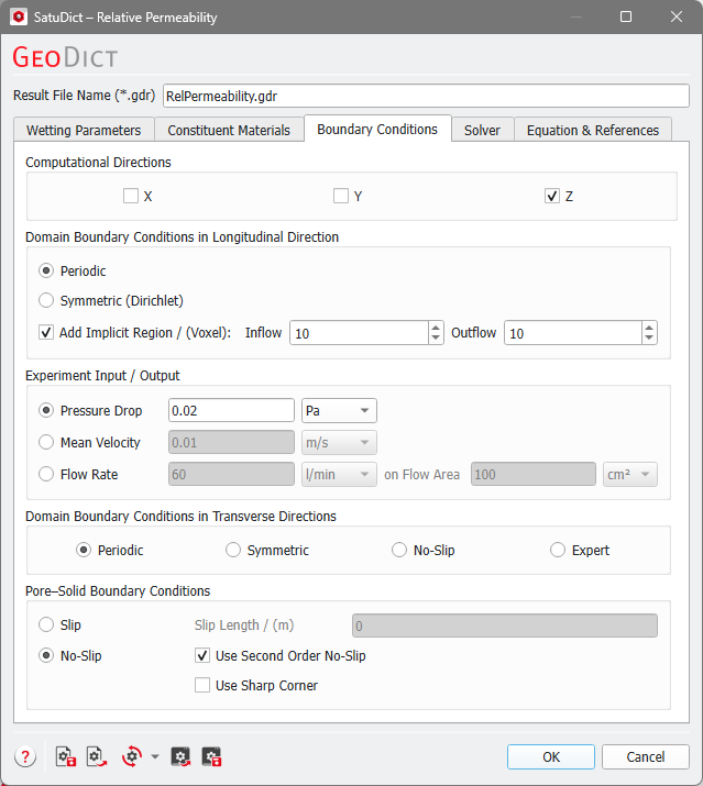
The Boundary Conditions tab is divided into five panels: Computational Directions, Domain Boundary Conditions in Longitudinal Direction, Experiment Input / Output, Domain Boundary Conditions in Transverse Direction,and Pore-Solid Boundary Conditions.
Note! The parameters are very similar to the parameters in the FlowDict Stokes(-Brinkman) command.
To simulate the flow through the domain, GeoDict solves a boundary-value problem. In the fluid-filled part of the domain, the flow is governed by a differential equation. The boundary values describe what happens at the boundaries, and are a necessary and important part of the problem description. Boundaries are the six faces of the cuboid (X-, X+, Y-, Y+, Z-, Z+), and the pore-solid walls within the structure.
For the six cuboid faces, FlowDict distinguishes between the domain faces in the computational direction (also called flow direction or longitudinal direction) and the domain faces in the two other space directions (called transversal or tangential directions). The computational direction is the direction in which pressure drop and flow rates are measured.
As Computational Directions, select the directions for which you want to calculate the flow. To obtain the full 3x3 permeability matrix and a pressure drop value for each direction in the results file, select all three directions.
For every selected direction, a boundary value problem is solved in which the Domain Boundary Conditions in Longitudinal Direction and the corresponding Experiment Input/Output are applied in the computational direction, and the Domain Boundary Conditions in Transverse Directions are applied on the other two space directions.
Any directions not selected will not be calculated and will be marked as 'unknown' in the permeability matrix in the Report tab of the result file.
The Domain Boundary Conditions in Longitudinal Direction can be checked to be Periodic or Symmetric (Dirichlet).
Use Periodic boundary conditions for periodically generated structure models and for non-periodic structures with high porosity. The structure is internally repeated periodically at the domain boundaries in the computational directions.
Use Symmetric boundary conditions for non-periodic structures if the percentage of solid voxels is high at the inlet. The solver treats the structure as mirrored at the domain boundaries in the computational directions.
The option to Add an Implicit Region is not available for Symmetric boundary conditions. The size of the implicit region in the computational directions is given in voxel, where the default added implicit inflow and outflow are 10 voxels, respectively.
Know how! The term implicit means that the region is only added by the solver internally. Thus, these regions do not contribute to the computed permeability and flow resistivity.
Note! A warning may appear when trying to run flow computations without adding an inflow region when the pore space at the domain boundaries in the computational directions is less than 50%.
The inlet and outlet are essential to avoid the possibility of closing the flow channels when the structure is periodically repeated. In the example shown below choosing periodic boundary conditions in the direction of the flow without adding an implicit region results in the flow channels being artificially closed.
To open the channels and enable flow, you can either add an inflow and/or outflow region, or select symmetric boundary conditions. However, when possible, we recommend using periodic boundary conditions, as these require less computational memory and take less time to run.
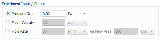
In the Experiment Input / Output panel select which property is prescribed in the computational direction. This will also define the property that will be computed. You can prescribe the Pressure Drop and obtain the Mean Velocity as result. Alternatively, you can prescribe the Mean Velocity or the Flow Rate and obtain the Pressure Drop as result.
This selection corresponds to the typical experimental setup, where you either apply a constant pressure drop over the media and measure the through flow rate or you apply a fixed pump flow rate and measure the resulting pressure drop over the media.
The Pressure Drop is the difference between the inflow and outflow pressures.
The Mean Velocity is the average speed of the flow in the positive direction, i.e., from Z- to Z+ if the Z-direction is the computational direction.
The Flow Rate on Flow Area is a volumetric flow rate. It is the fluid volume which passes per unit time through a given area.
For each property, the desired unit can be selected from the pull-down menu.
It is possible to use the Mean Velocity or the Flow Rate as input because the Stokes(-Brinkman) equation is linear. Thus, the solver can prescribe a pressure drop () and compute a mean velocity (). This mean velocity is not the desired mean velocity () entered in the Experiment Input / Output panel. Therefore, the velocity and pressure field are rescaled by . Then, the pressure drop () is calculated by
(334)
For example, if the desired velocity is twice the mean velocity used by the solver, the computed pressure drop is doubled to obtain the pressure drop corresponding to the desired mean velocity.
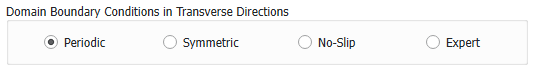
The Domain Boundary Conditions in Transverse Directions can be Periodic, Symmetric, No-Slip, or Expert.
With Periodic boundary conditions, the structure is repeated in the transverse directions.
With Symmetric boundary conditions, the structure is mirrored at the domain boundary. The LIR and EJ solver solve the symmetric boundary condition by using Neumann (or zero flux) condition at the domain boundary.
With No-Slip (or Encase) boundary conditions, the domain boundary is treated as closed by solid material. When No-Slip is used, the solver internally adds a one-voxel layer in the required direction and solves with periodic boundary conditions. This is effectively equivalent to solving the structure with casing at both sides in the transverse direction. So, the structure size in the corresponding transverse direction becomes enlarged by one voxel internally.
With Expert, it is possible to define different boundary conditions for each side in each computation. The boundary conditions in the two directions transverse to the flow can also be different by checking Expert boundary conditions. For example, when the fluid is chosen to flow in the Z-direction, the boundary conditions could be chosen to be No-slip in X-direction and Symmetric in the Y-direction.
The Slip Length allows to include sliding effects in the flow simulation. Sometimes the permeability of gases can be somewhat different from the permeability of liquids in the same media. One difference is attributable to "slippage" of gas at the interface with the solid when the gas mean free path is comparable to the pore size.
The default setting No-Slip corresponds to a flow velocity of zero along the structure.
Two settings are available for the No-Slip boundary condition. UseSecond Order No-Slip is activated by default. This sets the tangential velocity to zero at the center of the voxel surfaces and uses a second order approximation of the velocity field. The first order setting, which is used when the box is left unchecked uses a linear approximation (Harlow-Welch, 1965).
Use Sharp Corner can be used for digital rocks where permeability is usually overestimated or cases where voxels represent exact geometry. Activating it sets the tangential velocity to zero at the voxel corners. When the box is unchecked the default Round Corner is applied, which should be used for structures with round obstacles like fibers or grains.
Slip with a non-zero Slip Length simulates the sliding of the fluid along the solid, increasing the fluid mean flux and thus, the permeability of the structure. This option might be used when it is realistic for a given physical material. Currently, the same slip length value must be set for all materials in the structure.
In earlier releases, this feature worked correctly for axis aligned walls only, but since GeoDict 2020 the expression of the slip velocity, which assumes the slip velocity proportional to the shear stress at the surface, is reformulated for different velocity components when the angle of fiber surface is known, and reimplemented in the flow solver. Thus, direct simulation of the slip flow is possible.
(335) No flow into solid
(336) Slip flow along solid
Here, is the fluid flow velocity as it was introduced in Darcy's law and the Stokes equation, is the normal direction to the solid surface, is the fiber surface, is the Slip Length and is any tangential direction with . For the same pressure drop, the computed velocities for slip boundary conditions are higher than for no-slip boundary conditions. Conversely, for a given velocity or equivalently, a given mass flux, the pressure drop is lower when computed with slip boundary conditions.
For a straight channel structure, the two slip flow equations above become:
(337) Slip flow in straight channels
In this following example figure, the gray solid serves as a wall for a straight channel. To obtain the flow velocity along the solid () a coordinate system is defined by the solid orientation.
For a Slip Length of zero (), the graph that describes the flow velocity in dependence of the distance to the solid surface, would start at the surface of the solid. However, for a positive Slip Length () it is shifted into the solid by . Thus, the flow velocity is defined.


 Domain Boundary Conditions in Longitudinal Direction