Both LIR and EJ solve the Poisson equations by an iterative approach. The basic idea of an iterative method is to:

1. Start with some initial guess for the unknown values.
2. Improve the current values in each iterative step.
3. Repeat the iterative process until one of the stopping criteria (Error Bound, Tolerance, Residual, Maximal Iterations or Maximal Run Time) occurs.

For the EJ solver, select either Tolerance (recommended default) or Residual as stopping criterion. For the LIR solver, select Error Bound (recommended default) or Tolerance as stopping criterion.

Tolerance detects if the iterative process becomes stationary. This occurs when the change in the conductivity value from iteration to iteration becomes extremely small. If the relative change is smaller than the value entered for Tolerance the iteration is stopped.

When the Residual stopping criterion is used, the iteration is stopped if the solution satisfies the equation up to the required accuracy.

The default stopping criterion of the LIR solver, Error Bound, uses the result of previous iterations, and predicts the final solution based on linear and quadratic extrapolation. The solver stops if the relative difference regarding the prediction is smaller than the specified error bound. The stopping criterion recognizes oscillations in the convergence behavior and prevents premature stopping at local minima or maxima. A damped convergence curve is fit through the oscillating curve and the solver stops then regarding the damped convergence curve.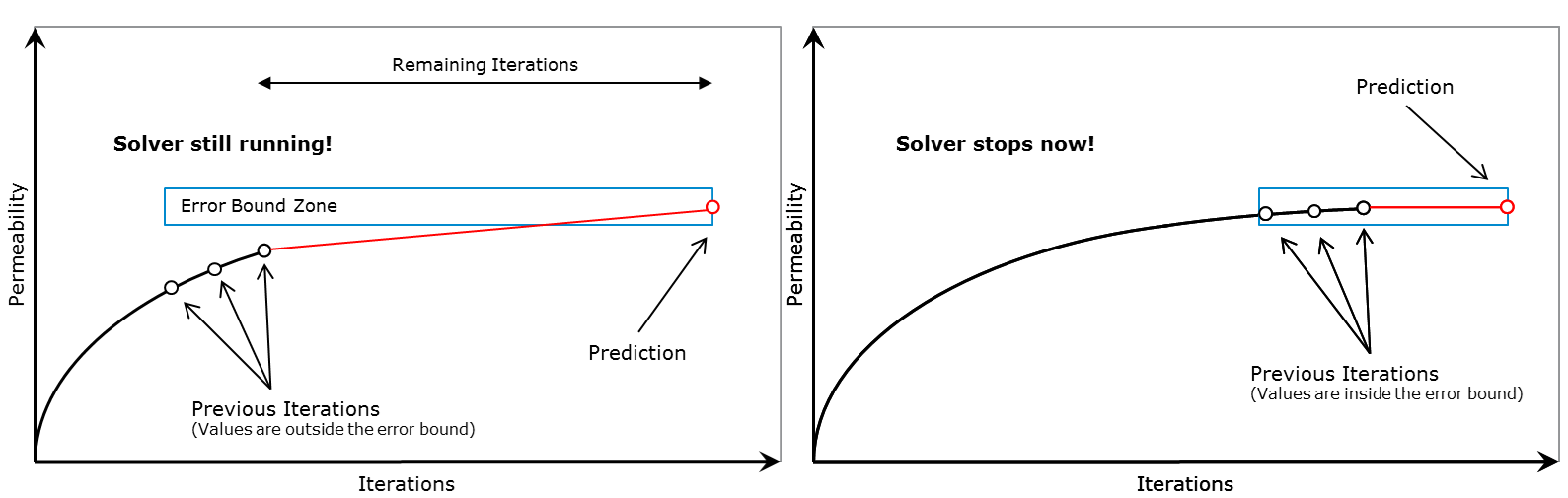

When the solver stops because the Maximal Iterations value or Maximal Run Time has been reached, no guarantee on the quality of solution can be given. Following possibilities might help:

• Check the corresponding .log file to see how large the residual values and conductivity increase are. If these values are already very close to the desired result, you may decide to use the current result.
• Double check the structure and parameter values. Unphysical parameters or too rough resolution of the structure (leading, e.g., to artificial unconnected components) can cause an iterative solver to fail.

Which stopping criterion has occurred, can be seen in the Result Viewer of the GeoDict result file (*.gdr) under the Results Map tab.

The calculations run by the solvers can be restarted from intermediate results, and the interval between auto-saves can be configured from the value entered in Restart Save Interval (h).

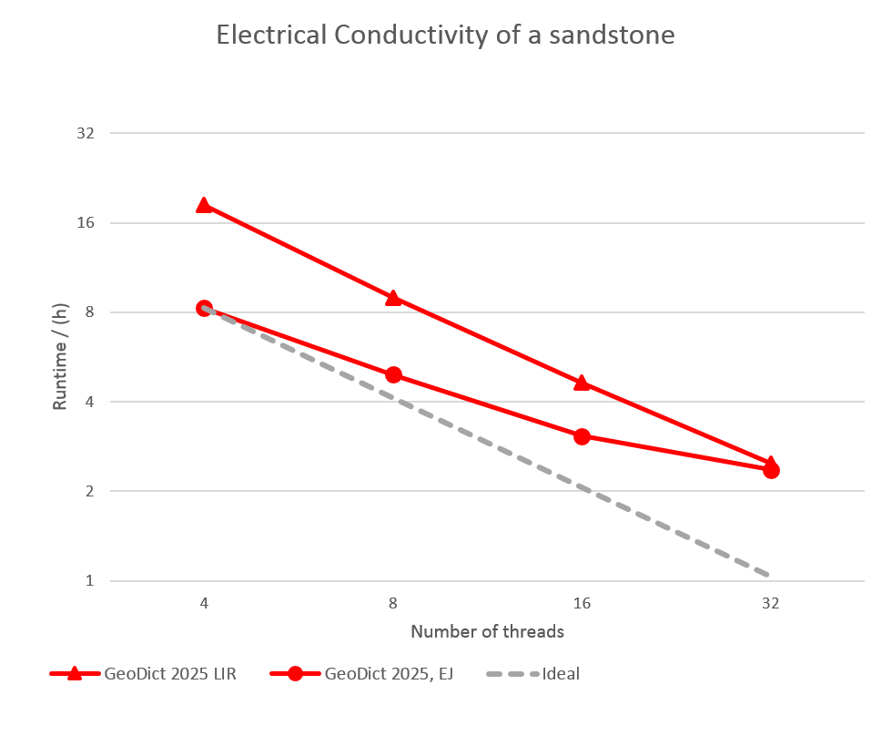
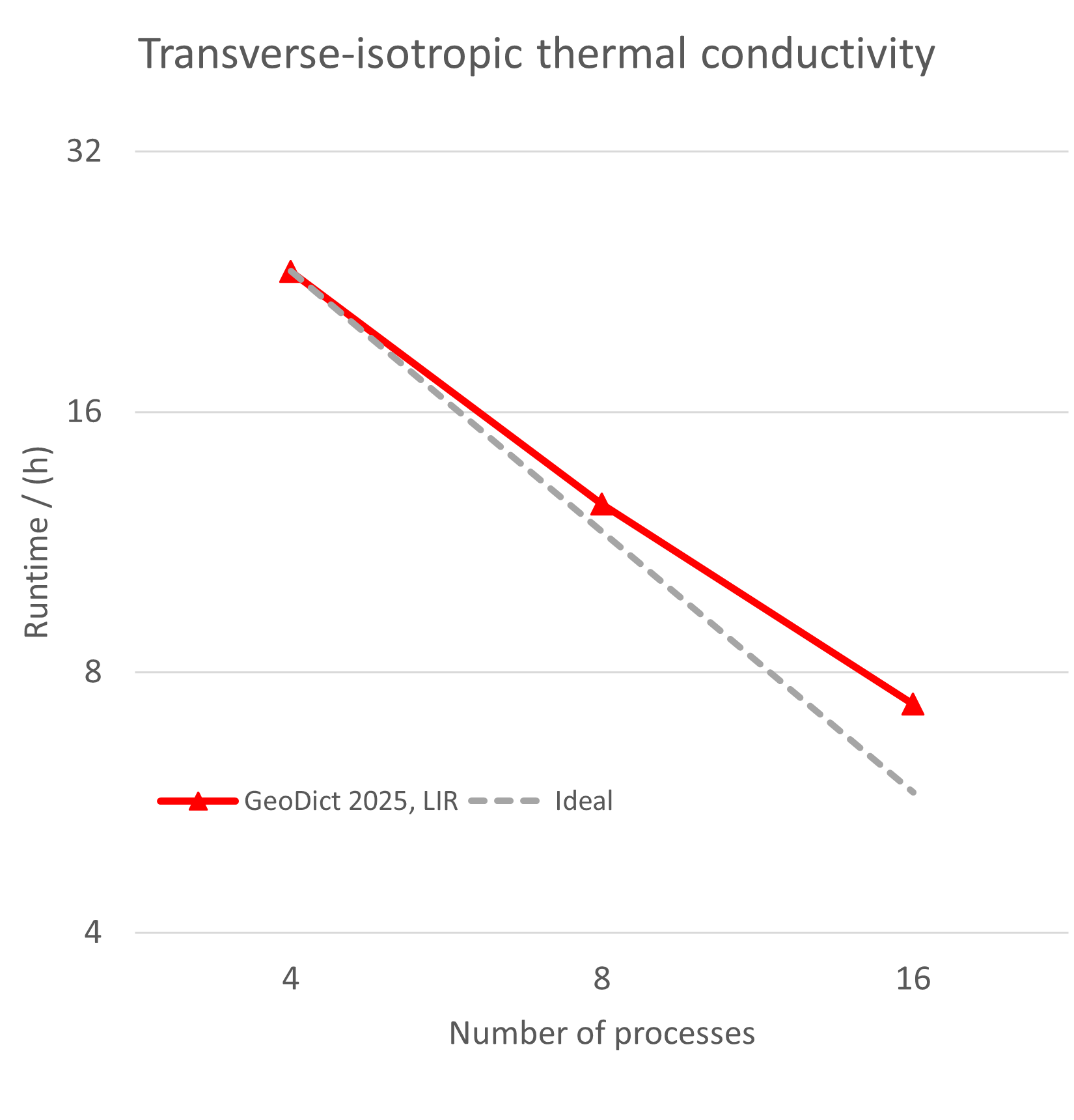
Depending on the purchased license, the simulation process can be parallelized.

The Parallelization Options dialog box opens when clicking the Edit... button, to choose between Sequential, Parallel (Shared Memory), Automatic Number of Threads, and Cluster for EJ, and Sequential, Parallel (Shared Memory), and Automatic Number of Threads for LIR.

For details on how to set up und run parallel computations, consult the High Performance Computing handbook.

Parallelization Benchmark Results Two examples of parallelization benchmark results for ConductoDict are shown here. Both benchmark computations were run on a server with 2xIntel E5-2697A v4 processors with 16 cores each, running with a maximum of 3.60 GHz, and 1024 GB RAM. The first example is the computation of the electrical conductivity through a synthetic X-ray tomography data of a sandstone structure (Mattila et al. 2016).The structure has a porosity of 13.6% and a size of 2048x2048x2048 voxels. The electrical conductivity of the structure, for pores filled with brine, is computed with the EJ and the LIR solver. For sandstone, an electrical conductivity of 1e-08 S/m and for the brine of 5 S/m is used as input values. The following figure shows the runtime for a different number of processes to compute the electrical conductivity of the structure of 0.1137 S/m with an error bound of 0.001 for LIR and of 0.1135 S/m with a tolerance of 0.001 with EJ solver. For both solvers, the ideal speedup, i.e. getting half of the runtime for twice the number of processes, is also shown. The speedup for LIR solver is close to the ideal one, which is usually not possible to reach for real life examples. The speedup of EJ differs more from the ideal one. For both EJ and LIR, the performance in GeoDict 2025 is comparable to the one in GeoDict 2024. The memory requirement for this example is 233 GB when LIR is used with the option of speed optimization, and is 239GB when EJ is used. The second benchmark is the computation of transverse isotropic thermal conductivity in a gas diffusion layer (GDL). The structure size is 4096x4096x512. A portion of the structure, of size 512x512x512 voxels, is shown in the figure below. The synthetic GDL, created with GeoDict, consists of 7% carbon fibers and 4% binder. The transverse isotropic thermal conductivity of 0.3 W/(mK) in both in-plane directions of the GDL and of 0.053 W/(mK) in through-plane direction is computed with the LIR solver with an error bound of 0.01. The following thermal conductivities for the different materials of the structure where used as input for the computation. Material Thermal Conductivity W/(mK) Fibers, in fiber direction 10 Fibers, orthogonal to fiber direction 2 Binder 1 Air 0.0257 Runtimes for a different number of processes are shown in the following figure. Again, the speedup of the LIR solver is close to the ideal one. For this example, LIR requires 259 GB memory.

In some situations, it may be useful to re-use previously computed results and, thus, reduce the runtime of the conductivity computation. Typical examples would be non-sufficient accuracy of some computation, when it is suspected that more iterations may improve the quality of the result.

To use some previously computed result, Restart from .gdr File can be checked and Browse used to search for the file.

Note that the structure used for restarting for both the current and the restart result file, must be the same. If this is not the case, an error message is displayed.

Checking the Discard PDE Solver Files box causes the deletion of all intermediate computation files. While having the benefit of saving storage place, discarding *.pde solver files has also the side effect of disabling the 3D visualization of the results.

Of course, the contents of the result file (*.gdr) are not discarded even in this case.

If one of the constituent materials has a transverse isotropic or orthotropic material law, a local orientation is needed to compute the conduction. There are three different choices how to determine the local orientation.

The standard case is to use the orientation defined by the local orientation of the GAD objects, e.g. the direction of a fiber.

However, if the current structure was not generated using one of the structure generation modules, but imported from a 3D image, GAD object information is not available. In such a case, the local orientation must be estimated from the image first, e.g. by using FiberFind or GrainFind. It is then possible to load the local orientation from a file generated by one of those modules:

Last, one can simply use the coordinate system:

In this case, the entered conductivities are the conductivities in the X, Y, Z space directions:

If contact resistances between objects of the same material have been set in the Constituent Materials tab, GeoDict must be able to distinguish between different objects of the same type. This can be done in two different ways.

The standard approach is to use the GAD information available for the current structure:

Such information is available if a green dot is shown in front of GAD Objects in the Project Status section (left side of the GUI).

A red dot might be shown if the current structure was not generated using one of the structure generation modules but imported from a 3D image. Then, GAD object information is not available, and the structure must be segmented into separate objects first, e.g. by using FiberFind or GrainFind. It is then possible to load the segmentation results from a file generated by one of those modules:

Please note that the Object Mode is only required when the contact resistance is between the same material IDs. No object information is necessary if all the contact resistances are between different material IDs.

Additional 3D data can be added to the solution .hht files for visualization or later analysis. For thermal conductivity computations, Write Heat Flux into Solution File stores the flux in the three coordinate directions, allowing a detailed analysis of the flux field.

The memory requirements increase when selecting this option.

Click on Advanced Options to expand the dialog:

Analyze Geometry

Analyze Geometry is checked by default to enable a geometry analysis before the solver runs to know if a through path exists.

Click on Advanced Options to expand the dialog: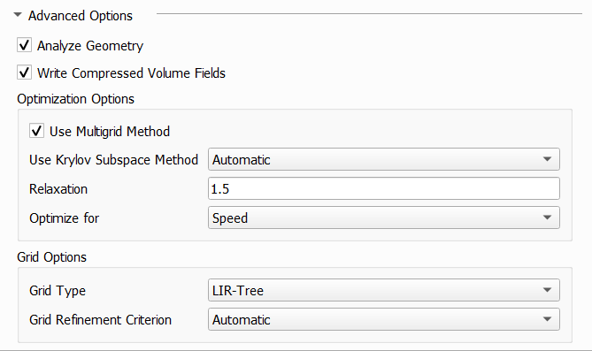

Analyze Geometry

Analyze Geometry is checked by default to enable a geometry analysis before the solver runs to know if a through path exists.

Write Compressed Volume Fields

If the option Write Compressed Volume Fields is checked for LIR solver then the adaptive grid structure is used as compression method for writing out .hht files. This option allows to save 80-90% space on hard drive.

The runtime for writing .hht files is also reduced significantly. If the option Write Compressed Volume Fields is not checked then a usual regular grid is used for writing out .hht files.

Use Multigrid Method

The Multigrid method was introduced to speed up the computation and reduce the runtime significantly. The main idea of Multigrid is the usage of multiple coarser adaptive grids to speed up convergence behavior but requires only a little more memory.

The method is available to solve the Stokes and Stokes-Brinkman equations in FlowDict as well as for solving diffusion, thermal and electrical conduction in DiffuDict and ConductoDict and is enabled by default.

Use Krylov Subspace Method

Depending on the structure and the corresponding material parameters, a significant speedup of the LIR can be achieved by using the BiCGstab method to compute the solution. Using the BiCGstab method approximately doubles the amount of RAM needed for the computation.

When Use Krylov Subspace Method is set to Automatic, GeoDict decides based on structure, material parameters and boundary condition which method is expected to be faster and uses this method. In case that the Krylov subspace method (BICGstab) is used, the Relaxation is also chosen automatically.

Alternatively, the user may also explicitly enable or disable this method.

If the ratio of the largest and smallest conductivity within the structure (i.e. high contrast) is large (approx. > ), usage of the Krylov method is recommended.

For structures without a high conductivity contrast, the usage of this option is not recommended.

Relaxation

Depending on the material parameters and geometry of the structure, the underlying mathematical problem can vary in complexity, thus influencing the behavior of the solver. The iterative method uses the Relaxation number to adjust it from Stable (with smaller number chosen, which results in higher number of iterations, slower time stepping, and longer solver run times), to Fast with higher number chosen, which makes the solver run less iterations but implies the risk that the solver does not converge.

For the LIR solver, this balance is managed through the Relaxation parameter. The value should be between 0 and 2. For relaxation values smaller than one (<1.0), the simulation is more stable. For relaxation values larger than one (>1.0), the simulation is faster.

Optimize for

The LIR solver can Optimize for speed or memory.

If Speed is chosen, the solver constructs additional optimization structures. The runtime decreases by up to 30% but requires up to 50% more memory compared to the other option. If Memory is chosen, then the runtime increases by up to 40% but the solver requires up to 50% less memory.

Grid Type

The Grid Type decides what kind of tree structure is used for the simulation.

The default option is LIR-Tree and should always be used. The solver uses an adaptive tree structure called LIR-tree and needs up to 10 times less runtime and memory compared to the Regular Grid option.

Grid Refinement Criterion

The solver can analyze the velocity and pressure field during the computation and improves the adaptive grid in places where more accuracy is needed. The LIR solver splits cells where a high velocity-gradient or high pressure-gradient occurs. The analysis is enabled if the Grid Refinement Criterion option is set to Automatic or Manual.

If the Grid Refinement is set to Automatic, the solver chooses the Number of Grid Refinements and Threshold for Grid Refinement automatically.

If the Grid Refinement Criterion is set to Manual, you can enter the parameters manually.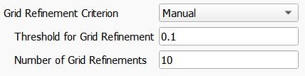

The Number of Grid Refinements controls how many velocity-based and pressure-based grid refinements are allowed during the simulation. The value should be between 0 and 10. Velocity-based and pressure-based grid refinements may increase the number of iterations, runtime, and memory requirements.

The Number of Grid Refinements can be zero in most of the cases and should be greater than zero if a flow simulation is done on a structure with a very long inlet and outlet, for pleated filter structures, or for Navier-Stokes simulations.

Refinement is done in the regions with high-velocity gradient or high-pressure gradient. Cells are split where the current velocity gradient (or pressure gradient) is greater than the Threshold for Grid Refinement multiplied by the maximal velocity gradient (or pressure gradient). This threshold must be between 0.0 and 1.0. The recommended value range is between 0.05 and 0.1.