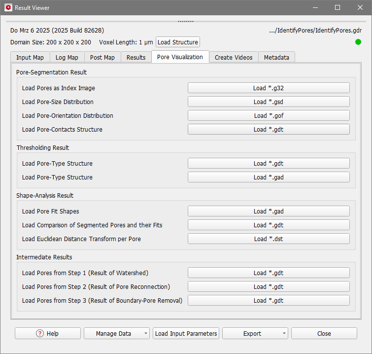
In the Pore Visualization tab you can import saved structures and computed volume fields which illustrate the pore identification process and its results.
Several options are available for the visualization of the different steps of Identify Pores and for the evaluation of the quality of the results. Some options might be unavailable, depending on the previously chosen parameters in the Identify Pores dialog (Output Options tab). The visualization options are grouped into panels.

|
Note! For the 3D visualization of the volume fields, reduce the visibility (in the View Controls) to the pore space of the structure because most values in the solid parts are zero.
|
Pore-Segmentation Result
In the first panel, several options for the analysis of the identified pore shapes are available.
 Load Pores as Index Image
With Load Pores as Index Image, all identified pores are assigned to a unique 32-bit color and can be investigated in the Visualization area. The 2D-view of *.g32 files is particularly suited for visual analysis of the correct segmentation.
|
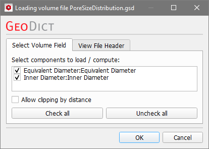
Load Pore-Size Distribution
This file is only available if Save Pore-Size Distribution (Volume-Equivalent Diameter) as *.gsd has been checked in the Output Options tab and contains the Equivalent Diameter field, which is the diameter of a sphere with the same volume as the pore.
If Save Inscribed-Sphere Diameters and Sheppard Sphericities was checked, the *.gsd file additionally contains the fields of the Inner Diameter, which is the diameter of the largest sphere that can be fitted inside the pore.
In the example below, the Boundary-Pore Removal was activated, thus the pores touching the domain boundary have diameter zero as they are excluded from the analysis.
|
Note! When you selected scalar values under GSD Field Choices in the post-processing widget, you can load the created *.gsd file here.
|
|
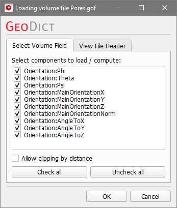
Load Pore-Orientation Distribution
This file is only available if Save Pore-Orientation Distribution as *.gof has been checked in the Output Options tab.
Several fields are saved in this file, e.g., the Euler Angles are available.
|
Load Pore-Contacts Structure
This file is only available if Save Pore-Contacts as *.gdt has been checked in the Output Options tab.
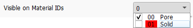
The pores have Material ID 01, while the contacts have Material ID 02.
|
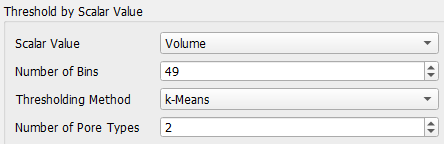
Thresholding Result
As explained in the previous topic, you can classify the pores by Thresholding a scalar value. For this example the default Threshold settings were used, where the pores are divided into two types based on the volume.
If you change the threshold settings, the pore-type structure will be recomputed.
Load Pore-Type Structure as *gdt
The pore-type structure saved in *.gdt format contains the identified pores with different Material IDs for the different pore types. The small pores are assigned to Material ID 01 and the large pores are assigned to Material ID 02.
|
Load Pore-Type Structure as *.gad
The pore-type structure saved in *.gad format contains the fitted ellipsoids with different Material IDs for the different pore types. The small pores are assigned to Material ID 01 and the large pores are assigned to Material ID 02.
|
Shape-Analysis Result
Load Pore Fit Shapes
With Load Pore Fit Shapes, load the *.gad file of the fitted ellipsoids for the individual pores.
|
Load Comparison of Segmented Pores and their Fits
To evaluate the performance of the pore identification with the chosen options use Load Comparison of Segmented Pores and their Fits. The identified pores, their best-fit shapes, and their overlap are shown as different materials (Original, Fit, and Overlap). Also have a look at the example in the topic Pore-Shape Analysis.
|
Load Euclidean Distance Transform per Pore
This file is only available if Save Euclidean Distance Transform per Pore as *.dst has been checked in the Output Options tab.
During the Identify Pores algorithm, first a Euclidean Distance Transform (EDT) and based on the results a Watershed transformation are performed. You can load the result of the EDT as volume file by clicking Load *.dst.
|
Intermediate Results
Results from the identification steps are loaded in the Intermediate Results panel.
Load Pores from Step 1 (Result of Watershed)
With Load Pores from Step 1 (Result of Watershed), the segmented pores after the Watershed transform are shown without any post-processing. Depending on the structure and the chosen Minimal Pore Diameter, this step might already be good enough to identify the pores. Otherwise, this option is useful to check the initialization options – mainly if the Minimal Pore Diameter was chosen correctly for the analyzed pore space.
|
Load Pores from Step 2 (Result of Pore Reconnection)
This file is only available if Reconnect Fragmented Pores has been checked in the Pore Segmentation tab.
By clicking Load Pores from Step 2 (Result of Pore Reconnection), the pores after the Pore-Fragment Reconnection are loaded in GeoDict. This way it can be assessed whether the chosen value for Interface Threshold suits the analyzed pore space.
|
Load Pores from Step 3 (Result of Boundary-Pore Removal)
This file is only available if Remove Pore Fragments at Domain Boundary has been checked in the Pore Segmentation tab.
Click Load Pores from Step 3 (Result of Boundary-Pore Removal) to import the identified pores resulting from the removal of pore fragments at the domain boundary. This will be the basis structure for the fitting of the ellipsoids.
|