After the solver run has finished, the Result Viewer opens immediately. The results are similar as seen for the Capillary Pressure Curve, but some more options are additionally available.

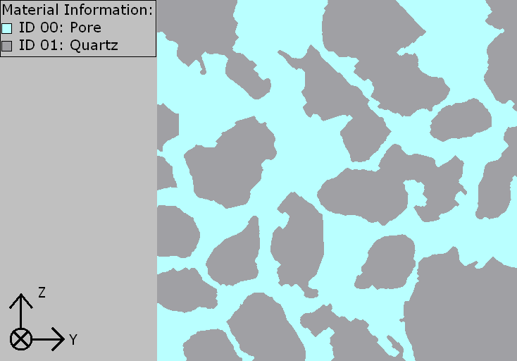
In the example, the calculations of Mercury Porosimetry & Capillary Pressure are run on a porous structure with 54% SVF, originated from Berea sandstone. A 2D cross-section view of the structure is shown below.

The Results tab is the central point analysis of the results. It is grouped in three subtabs: Report, Plots and Map. The Report tab shows diameters, curvatures and capillary pressure values for each saturation step. The Plots tab contains plot options for the analysis of the results. The Map tab contains all resulting data from the run. This data is the basis for the tables in the Report tab and for the plots in the Plots tab.

Load additional files to visualize the results in the Data Visualization tab.

Report

For a typical capillary pressure result file, the table shows the Saturation of the invading fluid, the saturation of the displaced fluid, the Mean curvature and the calculated corresponding Capillary pressure for every step (pore size). The mean curvature approximates the fluid-fluid interface curvature.

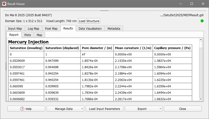
For computations with the Contact Angle Method Constant Contact Angle also the Pore diameter is shown in the table. This is the diameter of the pores filled in this saturation step.

Plots

Pressure-Saturation

Observe the tabular results of the Report subtab as a diagram in the Pressure-Saturation subtab.

On the left, the Post-Processing Widget allows you to fine-tune this graph. Collapse the Post-Processing Widget by pulling it to the left.

Select the Graph Type (Pressure over Saturation or Saturation over Pressure), Phase Selection (Invading Fluid or Displaced Fluid), Saturation Unit (Relative or Absolute) and Reference Volume (Pore Space or Total Sample Volume). Check Invert Saturation to show the values of the saturation in decreasing order instead of increasing order.

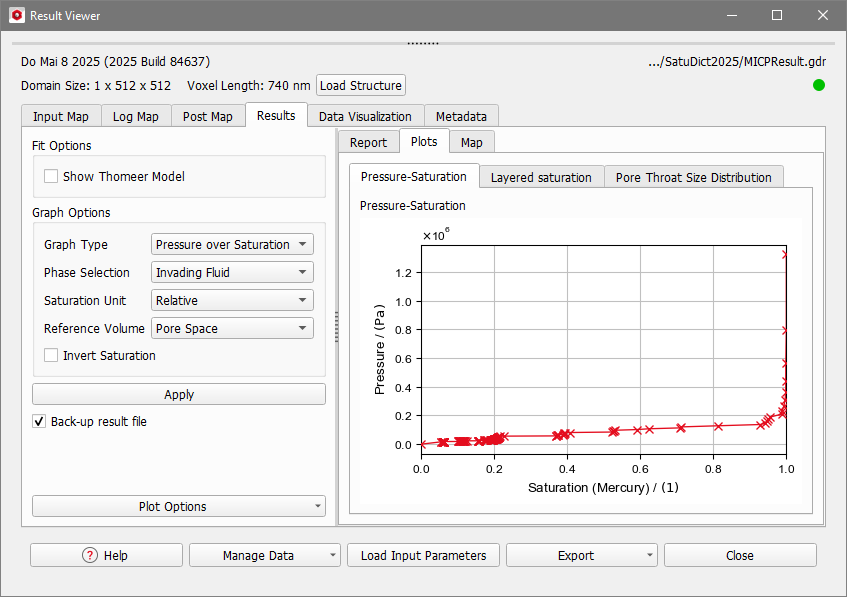
In the example, at the beginning of the injection process, the porous structure does not contain the invading fluid Mercury. As the pressure increases, the Mercury starts invading the structure and the saturation of the Mercury is increasing. By the end of the injection process, where the pressure is at its highest level, the structure is 100% saturated with Mercury.

If a Thomeer Model is fitted, this model can be shown by checking Show Thomeer Model under Fit Options.

Layered saturation

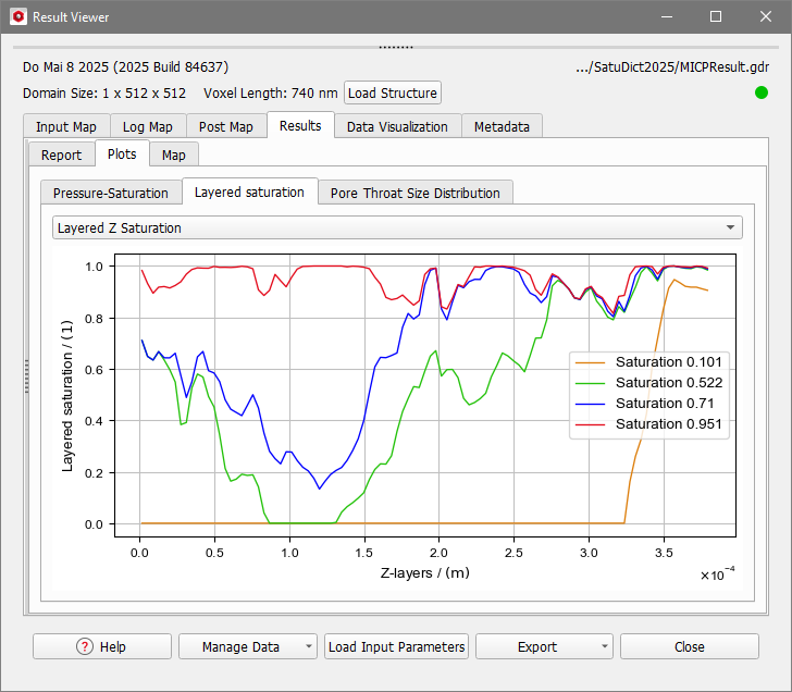
In the subtab Layered saturation, the saturation along each of the three axes (X-, Y-, and Z-axis) is shown.

From the drop-down menu choose the direction to observe. For each layer, the occupied space of the invading fluid relative to the pore volume of this layer is plotted. This can be done for several steps of the calculation, which corresponds to different saturations of the whole structure. By right-clicking into the plot area, the curves of different saturation steps can be selected.

Pore Throat Size Distribution

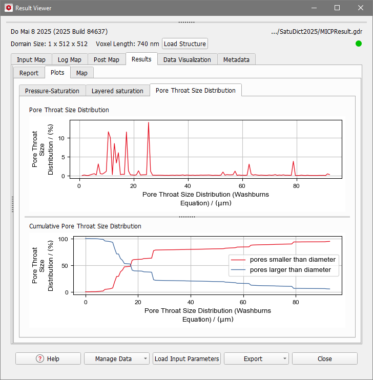
Using the Washburn / Young-Laplace Equation the resulting capillary pressure values are related to a Pore Throat Diameter. The resulting distribution is shown in two plots, which are very similar to the plots of PoroDict-Porosimetry.