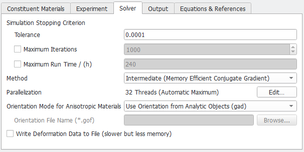
On the Solver tab, specify the settings for the FeelMath solver.

Simulation Stopping Criterion

The equations are solved by an iterative approach.

The iterative process is controlled by setting the values and activation for Tolerance, Maximal Iterations, and Maximal Run Time (h). The stopping criteria apply for each computational direction individually.

If multiple stopping criteria are selected, the first criterion that is reached causes the solver to stop.

The stopping criterion that has been reached can be viewed in the Result Viewer of the GeoDict result file (*.gdr) under the Results Report tab.

Tolerance

Maximum Iterations and Maximum Runtime

Method

For the FeelMath-Deformations solver, three different iterative methods are available: Fast (Conjugate Gradient), Intermediate (Memory Efficient Conjugate Gradient), and Memory Efficient (Neumann Series).

The Fast method converges faster, especially for strongly varying material parameters and nonlinear material laws (as, e.g., plasticity or damage), but needs about four times as much memory as the Memory Efficient method.

The Intermediate Method needs approximately 40 % less memory than the Fast method but is slower. The Estimate Memory button in the ElastoDict section can be used to decide which method is applicable for the current structure on the available computer.

In general, it is recommended to use the default (Memory Efficient Conjugate Gradient) or the Conjugate Gradient method. The Neumann Series method should only be used if the memory is not sufficient for the other methods.

Parallelization

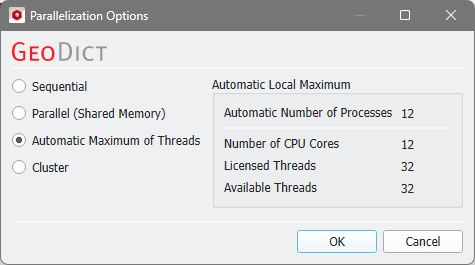
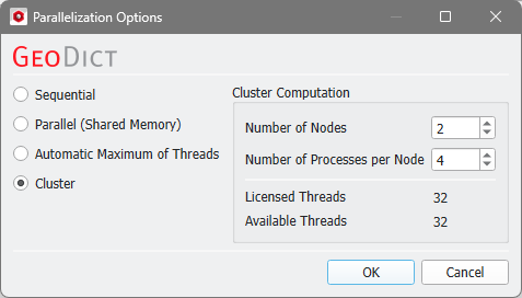
Control how many threads are used for the computation. Parallelization is possible if your license and hardware allow it.

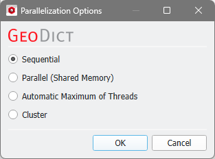
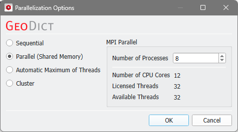
The Parallelization Options dialog opens when clicking the Edit button and you can choose between Sequential, Parallel (Shared Memory), Automatic Maximum of Threads, or Cluster (only available if EJ, SimpleFFT, or FeelMath were selected as solver).

The parallelization of the solvers is done with two technical methods: MPI Parallelization or Thread parallelization. The following table shows the support of both parallelization methods:

Depending on the used parallelization method, the Number of Processes (MPI parallel) or the Number of Threads (thread parallel) can be entered.

Sequential

Parallel (Shared Memory)

Automatic Maximum of Threads

Cluster

Orientation Mode for Anisotropic Materials

BatteryDict-Degradation can handle non-isotropic constituent materials. For these materials, an orientation must be additionally specified. If the analyzed structure consists of analytical objects (gad data), the orientation of these objects is used when Use Orientation from Analytic Objects (gad) is selected.

Alternatively, with Load Orientation Information from File (*.gof), orientation information can be loaded from a file. Such a file can be generated for example with GrainFind for granular structures. The third option, Use the Global XYZ-Coordinate System, allows to use anisotropic materials even if no orientation information for the structure is available. This makes sense only if the grains are all oriented directly according to the coordinate axis, which is usually not the case.

Write Deformation Data to File

For the computation of the deformed structures, intermediate data is computed which describes the displacement for each voxel. Before this computation, it is not clear how large this data will be, since a voxel in the original structure might be partially moved in multiple voxels in the deformed structure. Therefore, this data might not fit in the main memory of the computer. Due to this, it is possible to write the deformation data to a file on the hard disk by checking Write Deformation Data to File.

But note that writing and loading data from the hard drive is many times slower than writing and loading data in the main memory (even if the drive is an SSD). This causes a bottleneck, which can slow down the simulation.

If the data exceeds available RAM, you can store the deformation data on disk by enabling “Write Deformation Data to File. We recommend keeping this setting, and to select Write Deformation Data to File only if the simulation fails because the data does not fit into the RAM.