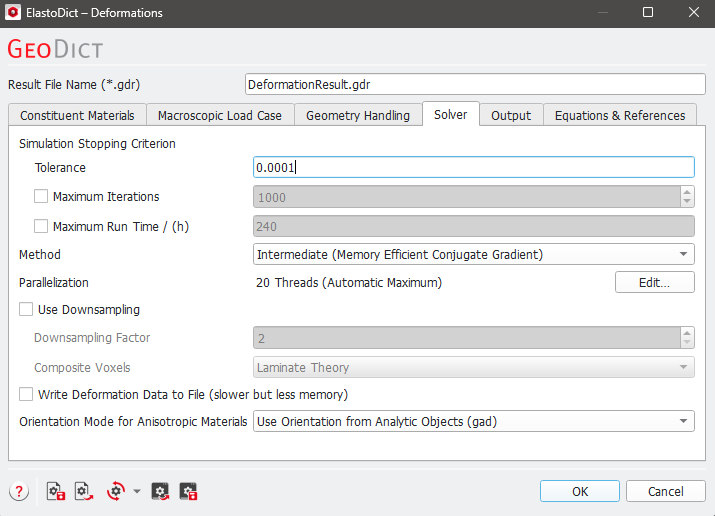
The iterative process of the solver is controlled by setting the values for Tolerance, Maximal Iterations, and Maximal Run Time (h). Only the tolerance must be set, the two other parameters are optional.

For each iteration step, the relative error of the current solution is computed. If this relative error is smaller than the given tolerance, the computation is finished. When there is doubt about the quality of the solution, decrease the tolerance value by a factor of ten for that solver. In general, it is recommended to keep the default setting for tolerance.

When the solver stops because the Maximal Iterations or the Maximal Run Time (h) are reached, the quality of solution might be doubtful since the requested accuracy is not achieved. Therefore, those two options are disabled by default and should only be selected if there are strong constraints on the allowed runtime.

For the FeelMath solver, three different iterative methods are available: Fast (Conjugate Gradient), Intermediate (Memory Efficient Conjugate Gradient) and Memory Efficient (Neumann Series).

Fast: here the CG method is used (Conjugate gradient method - Wikipedia), which is the fastest available approach in ElastoDict, especially for strongly varying material parameters and nonlinear material laws as, e.g., plasticity or damage. The convergence rate is proportional to the square root of the stiffness contrast. However, it needs up to 4 times more memory compared to the Memory Efficient method. We recommend using the Fast method whenever possible.

Intermediate: this is a memory efficient CG method, which needs approximately 40 % less memory than the Fast method but may be 20-30 % slower.

Memory Efficient: here the Neumann series is used. It is the most memory efficient method, but the convergence rate is proportional to the stiffness contrast in the materials and can therefore be low. This method should only be used for applications with a low stiffness contrast, or if the RAM is not sufficient.

For Deformations and Effective Stiffness, the Estimate Memory button is present in the ElastoDict section. When the structure of interest is shown in the Visualization area, clicking Estimate Memory calculates the memory needed for the computations based on the size of the structure and the parameters entered in the solver options. The Estimate Memory button can be used to decide which method is applicable for the current structure on the available computer.

The ElastoDict run can be accelerated by using multiple CPU cores. The Parallelization Options dialog opens when clicking the Edit... button, to choose between Sequential, Parallel (Shared Memory), Automatic Number of Thread and Cluster as well as MPI Parallel for Linux users.

When Sequential is selected only one thread is used for the computation.

Selecting Parallel (Shared Memory) runs the parallel computation with the specified Number of Processes on a shared-memory hardware. Then the maximum number of available processors and the maximum number of licensed parallel processes is shown in the dialog.

If Automatic Maximum of Threads is selected, the number of parallel processes is automatically selected for optimal speed, based on the CPU cores and licensed parallel processes. For up to eight Available Threads, all of them will be used. If more than eight threads are available, two cases might occur:

• The number of Available Threads is larger (or equal) than the Number of CPU Cores:
  • Then the maximum of eight and Number of CPU Cores divided by 2 is used.
• The number of Available Threads is smaller than the Number of CPU Cores:
  • Then the maximum of eight and number of Available Threads divided by 2 is used.

For users of Linux systems the solver supports the MPI parallelization method. The Parallelization Options dialog under a Linux system has the options MPI Parallel (Shared Memory)  and Thread Parallel (Shared Memory) as the parallelization can be done with MPI parallelization or Thread parallelization.

For details on how to set up and run parallel computations, consult the High Performance Computations User Guide.

Downsampling reduces the structure size by combining multiple voxels. By default, the Downsampling Factor is set to two – this means that 2x2x2 voxels are combined to one voxel. The material model used for each voxel in the downsampled structure is a combination of the material model (e.g., a Composite Voxel) of the original voxels. Since the simulated structure size is much smaller than the original structure, Downsampling allows to speed up the simulation and to quickly obtain results even on computers with little memory. This option should not be used if highest accuracy is required.

Downsampling Factor

In most cases, a Downsampling Factor of 2 is the best choice, but it can also be set to 4 if needed. Then, the computation will be faster, but the results could be more inaccurate.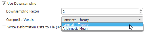

To be able to use downsampling, the features (e.g., fibers or grains) in each material ID must have a diameter of at least the Downsampling factor in voxels (e.g., 2 voxels for a Downsampling Factor of 2). Otherwise, the computation of the material properties might not work properly. Since GeoDict 2021, an error message is shown if all features in the structure are smaller than this diameter, and the simulation cannot be started.

Composite Voxels

Two different methods to compute the Composite Voxels during downsamling: Laminate Theory (the default), and Arithmetic Mean. When using Laminate Theory, the composite material properties are computed based on the laminate theory of composite materials. With this option, also direction dependent properties are represented correctly, which is important especially at the boundary between two different materials. With Arithmetic Mean, the material properties of the composite voxel are the average of the material properties of the original voxels. This method is less accurate, but the simulation might be more stable, especially if the structure contains many pores (as e.g., in foams). Nevertheless, it is recommended to keep the default Laminate Theory in most use cases for the higher accuracy.

For the computation of the deformed structures, intermediate data is computed which describes the displacement for each voxel. Before this computation, it is not clear how large this data will be, since a voxel in the original structure might be partially moved in multiple voxels in the deformed structure. Therefore, this data might not fit in the main memory of the computer. By checking the option Write Deformation Data to File, the deformation data will be written to the hard drive .

We recommend keeping this option disabled, and to select it only if the calculation of the deformed geometry fails because the data does not fit into the RAM. Writing and loading data form the hard drive is many times slower that writing and loading data in the main memory (even if the drive is an SSD). This causes a bottleneck, which can slow down the simulation.

ElastoDict can handle non-isotropic constituent materials. For these materials, an orientation has to be additionally specified. If the analyzed structure consists of analytical objects (gad data), the orientation of these objects is used when Use Orientation from Analytic Objects (gad) is selected.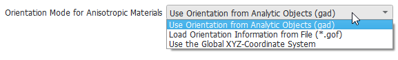

Alternatively, with Load Orientation Information from File (*.gof), orientation information can be loaded from a file. Such a file can be generated for example with GrainFind for granular structures.

The third option, Use the Global XYZ-Coordinate System, allows to use anisotropic materials even if no orientation information for the structure is available.