Click OK to input the entered parameters, and then click Run in the ConductoDict section to start the command. The results are immediately shown in the opening Result Viewer after the process is finished.

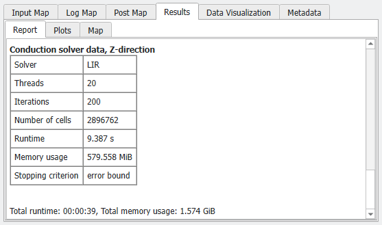
The Results - Report sub-tab displays the computed Thermal Conductivity tensor.

Also, for each computation, the solver, number of threads, number of iterations, number of cells (only for LIR), runtime, and stopping criterion are reported.

The Results - Plots sub-tab allows choosing different plots.

Under Temperature, the temperature gradient across the structure can be plotted. The plot shows on the y-axis the computed average temperature on each voxel layer.

Right clicking on the plot opens a small dialog box where you may choose to Edit Axis Settings.

In the dialog that appears, you may change the scale, ticks and labels of the X- and Y-axis manually, and set the position of the legend in the chart.  

Under HeatFlux, the mean heat flux and the standard deviation in each layer is plotted.

When all parts of the structure are conducting (example on the right hand side), the mean current density is constant, and the standard deviation shows in which parts of the structure material with higher conductivity is accumulated.

If non-conducting materials are present (example on the left-hand side), the mean current density varies and shows where the bottlenecks are.

Under Convergence, the plot of the Conductivity at given Iteration values is charted for the selected directions. Selecting the direction from the pull-down menu, it is possible to see graphs of the convergence of the iterative solver for each of the computed directions.