The equations are solved by an iterative approach.

The iterative process is controlled by setting the values and activation for Enter value, Maximal Iterations, and Maximal Run Time (h). The stopping criteria apply for each computational direction individually.

If multiple stopping criteria are selected, the first criterion that is reached causes the solver to stop.

The stopping criterion that has been reached can be viewed in the Result Viewer of the GeoDict result file (*.gdr) under the Results Report tab.

The default stopping criterion of the LIR solver, Error Bound, uses the result of previous iterations, and predicts the final solution based on linear and quadratic extrapolation. The solver stops if the relative difference between computed and predicted solution is smaller than the specified error bound. The stopping criterion recognizes oscillations in the convergence behavior and prevents premature stopping at local minima or maxima. A damped convergence curve is fit through the oscillating curve and the solver stops then regarding the damped convergence curve.

If the Krylov method (under LIR - Advanced Options) is activated, Enter valuethe definition of Error Bound is somewhat different. Here, no prediction is made, instead the continuity between neighboring cells and the conservation of mass is checked. The maximal value is normalized by the mean flow and if this value is smaller than the Error Bound the simulation stops.

The Tolerance stopping criterion, the default stopping criterion for EJ, looks for stagnation of the method when the process becomes stationary, i.e. the improvement in the permeability value becomes extremely small from iteration to iteration.

In each iteration, the solver checks for the current computed value against the values of the last 100 iterations if there are any changes.

The computation is stopped if the maximal relative change is smaller than the value entered for Tolerance. When there is doubt about the quality of the solution, decrease the Tolerance value by a factor of ten. The drawback of this criterion is that the solver sometimes might stop too early in case of slow convergence rate or at local extrema of oscillatory convergence curves.

Use the Maximum Iterations value or the Maximum Run Time (h) stopping criteria causes the solver to stop if the maximal number of iterations and/or the maximal run time (in hours) is exceeded.

When the solver stops because one of these criteria has been reached, no guarantee on the quality of solution can be given. In this case, a warning is printed into the report. The following possibilities might help:

• Check the corresponding .log file to see how large the residual values and permeability values are. If permeability values are in reasonable range and they do not have changed during the last iterations, you may decide to use the current result.
• Double-check the structure and parameter values. Unphysical parameters or too rough resolution of the structure (leading, e.g., to artificial unconnected components) can cause an iterative solver to fail.

The calculations run by the solvers can be restarted from saved intermediate result files and the interval between auto-saves can be configured from the value entered in Restart Save Interval (h).

Control how many threads are used for the computation. Parallelization is possible if your license and hardware allow it.

The Parallelization Options dialog opens when clicking the Edit button and you can choose between Sequential, Parallel (Shared Memory), or Automatic Maximum of Threads.

Selecting Sequential will not apply parallelization and only one thread is used for the computation.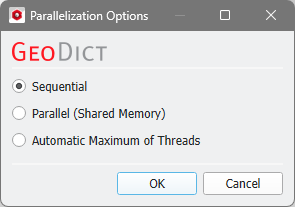

When Parallel (Shared Memory) is selected, the Number of Threads can be entered. Below, the Number of CPU Cores that the current machine has, the maximum number of Licensed Threads and the number of those licensed threads that are available (Available Threads) are shown in the dialog. Of course, the maximal number of parallel processes you can use, is the smallest of those three numbers.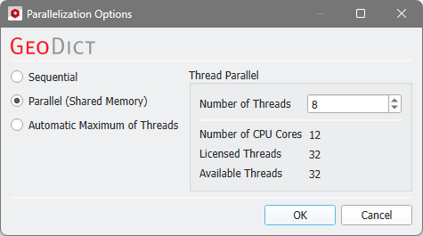

If Automatic Maximum of Threads is selected, the number of parallel processes is automatically selected for optimal speed, based on the CPU cores and licensed parallel processes.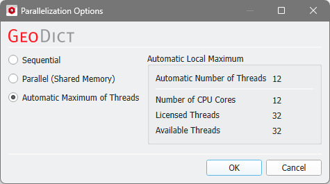

The Automatic Local Maximum of processes is automatically selected, which is the minimum of Number of CPU Cores, Licensed Threads, and Available Threads.

In some situations, it may be useful to re-use previously computed results and save a great amount of time by restarting the process from an existing GeoDict result file (*.gdr). Typical examples would be

• non-sufficient accuracy of some computation, when it is suspected that more iterations may improve the quality of the result,
• trying another boundary condition (e.g., Dirichlet instead of Periodic or other way around),
• continuing an iteration process,
• or using similar parameter values for the computation.

To restart and initialize the solver from a result file (*.gdr), check Restart from .gdr File and enter the name of a file, or Browse for it in the project folder.

When using Restart From .gdr File only the volume field (*.hht file) associated to the loaded *.gdr file will be used to continue the simulation.

No other parameters from the options dialog will be loaded from the *.gdr file, but it is possible to load them by clicking Load Parameters in the Result Viewer. This way the simulation can be continued while using the same settings as in the initial simulation.

Checking Discard PDE Solver Files causes the deletion of all intermediate computation files, such as log files and flow field files.

Only the content of the final GeoDict result file (*.gdr) is stored.

While having the benefit of saving hard disk storage place, discarding intermediate solver files has also the effect of disabling the 3D visualization of the results.

Checking Analyze Geometry performs an analysis of the geometry before the solver computations.

If no percolation path through the structure is found, the partial differential equation does not need to be solved, and a permeability of 0.0 is directly reported as the solution.

Furthermore, the solver operates on the whole structure, regardless of which parts are connected or unconnected. However, unconnected components are not transport relevant, thus the effort of solving in these parts is not necessary.

For these reasons, a geometrical analysis is routinely run to determine whether a through path exists. After the analysis is finished, unconnected components are removed from the computational grid.

This may speed up the computations but requires some time for the geometrical analysis, especially for very large structures. So if you know beforehand that there are no unrelevant parts or that the structure has been processed to eliminate them, the geometry analysis can be switched off by unchecking Analyze Geometry.

The LIR solver uses a very memory efficient adaptive grid structure for the simulations.

If the option Write Compressed Volume Fields is checked, then the adaptive grid is used as compression method for writing out *.hht files. This option allows to save 80-90% space on hard drive. The runtime for writing *.hht files is also reduced significantly. But the runtime for loading and uncompressing of compressed *.hht is increased by the amount of runtime that was saved for writing out compressed *.hht files.

If the option Write Compressed Volume Fields is not checked, then a usual regular grid is used for writing out *.hht files.

The Multigrid Method (see e.g. Wesseling, 2004) was introduced to speed-up the computation and reduce the runtime significantly. The main idea of Multigrid is the usage of multiple coarser adaptive grids to speed up convergence behavior but requires only little more memory.

The method is available to solve the Stokes and Stokes–Brinkman equations as well as for solving mechanics, diffusion, thermal, and electrical conduction and is enabled by default.

Another speed-up option to accelerate the convergence behavior of the LIR solver is called Krylov Subspace Method.

The runtime of the LIR solver depends on many different properties of the structure and the simulation parameters. The BiCGStab algorithm is used, which can reduce the runtime for challenging simulation very drastically.

Unfortunately, the Krylov method is not always faster than a simulation without the Krylov method and therefore we introduced an Automatic mode which uses some heuristics to choose the most efficient method based on structure, material parameters, and boundary conditions automatically. Of course, it is possible to explicitly enable (Enabled) or disable (Disabled) the method.

Depending on the material parameters and geometry of the structure, the underlying mathematical problem can vary in complexity, thus influencing the behavior of the solver. The more complex the problem is, the more stable the solver settings should be.

With the Relaxation number, the solver is adjusted from Stable (which results in higher number of iterations, slower time stepping, and longer solver run times), to Fast, which makes the solver run less iterations but implies the risk that the solver does not converge. The Relaxation is a parameter of the SOR method and must be between 0 and 2 to ensure convergence. For relaxation values smaller than one (<1.0), the simulation is more stable. For relaxation values larger than one (>1.0), the simulation converges faster.

The LIR solver can Optimize for Speed or Memory.

• If Speed is chosen, the solver constructs additional optimization structures. The runtime is decreased by up to 30% but requires up to 50% more memory compared to the other option.
• If Memory is chosen, the runtime is increased by up to 40% but the solver requires up to 50% less memory.

The Grid Type decides what kind of tree structure is used for the simulation.

The default option is LIR-Tree and should always be used. The solver uses an adaptive grid structure called LIR-tree and needs up to 10 times less runtime and memory compared to the Regular Grid option.

The solver can analyze the result field during the computation and improves the adaptive grid in places where more accuracy is needed. The LIR solver splits cells where a high gradient occurs.

The solver can analyze the computed field and refines the adaptive grid during the computation at locations where more accuracy is needed. The LIR solver splits cells where a high gradients occur when the Grid Refinement Method is enabled. In this case, the additional parameters Number of Grid Refinements, Allow Sub-Voxel Resolution, and Allow Grid Re-Coarsening become available.

Select one of the three available refinement methods from the drop-down menu.

When A Posteriori Error Bound is selected, the solver targets the specified accuracy Threshold. While the Error Bound (set as Simulation Stopping Criterion) determines the relative error in the solution of the linear system, A Posteriori Error Bound refers to the relative error estimated by comparing high-order and low-order discrete solutions. The accuracy Threshold refers to the relative error to the analytical solution and the value must be between 0.0 and 1.0.

Choosing Difference (Automatic) leads to computational cells being split when the difference in values between neighboring cells exceeds a certain Threshold. The solver automatically chooses all internal parameters based on the structure and simulation settings. For this option, cells are split where the current gradient is greater than the Threshold multiplied by the maximum gradient, where the threshold is determined automatically.

Selecting Difference (Manual) also causes the computational cells to be split when the difference in values between neighboring cells exceeds the specified Threshold. You can specify all parameters (Threshold and Number of Grid Refinements) for the grid refinement manually. For this option, cells are split where the current gradient is greater than the Threshold multiplied by the maximum gradient. The Threshold value must be between 0.0 and 1.0. The recommended value range is between 0.05 and 0.1.

Activate Reynolds Grid Refinement to use the local Reynolds number (Re) for adaptive grid refinement.

A grid cell is split if the local Reynolds number, i.e. the ratio between inertial and viscous forces exceeds the given threshold. The Reynolds number is defined as:

where is the density of the fluid (SI units: kg/m3), u is the velocity of the fluid (m/s), is the dynamic viscosity of the fluid (Pa·s or N·s/m2 or kg/m·s), L is a characteristic length (m). For the local Reynolds number, the size of the grid cell is used for the characteristic length.

The Number of Grid Refinements controls the maximum number of grid refinements that the solver can perform during the simulation. The value should be set between 0 and 10, where a value of 0 means that no grid refinements will be made. Grid refinements may increase the number of iterations, runtime, and memory requirements.

When Allow Sub-Voxel Resolution is enabled, the solver is allowed to split computational cells to sizes smaller than the voxel length.

This feature is beneficial for low-porosity structures for which the pore throats require finer resolution or for modeling fast Navier-Stokes flows with strong vortices.

Enabling this feature may increase the number of iterations, runtime, and memory requirements.

Check Allow Grid Re-Coarsening to allow the solver to automatically revert the grid refinement and coarsen the computational cells.

This means, grid refinement is done temporarily. Afterwards, the cells are merged as soon as accuracy is not needed anymore. This reduces the memory and runtime requirements.