Click OK to input the entered parameters, and then click Run in the FilterDict section to start the Filter Efficiency simulation.

The results are immediately shown in the opening Result Viewer after the simulation is finished.

Report

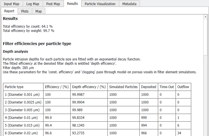
Under the Report tab, the following results are reported:

• The Total efficiency by count, computed as , where is the fractional filtration efficiency of a particle type and the count probability (Count % entered on the Particles→Size Distribution tab) of this particle type.

• The Total efficiency by weight, computed as , where is the fractional filtration efficiency of a particle type and the mass probability (Mass % entered on the Particles→Size Distribution tab) of this particle type.

In the Filter Efficiencies per Particle Type table below, for each particle type, the following values are given:

• The fractional filtration Efficiency.
• An estimated fractional filtration efficiency, called Depth Efficiency, determined by fitting an exponential decay function to the particle intrusion depth distribution (see the description of the Plots sub-tab below for details).
• The overall number of Simulated Particles of this type. Be aware that those numbers do not follow the size distribution entered on the Particles→Size Distribution tab, each particle type is simulated Number of particles per type times as entered on the Particles→Positioning tab.
• The number of those particles Deposited on the filter.
• The number of Time-Out particles, which are still in motion when the maximal simulation time is reached (Max time reached on the Filter Experiment tab).
• The number of particles that have arrived unfiltered in the Outflow area.

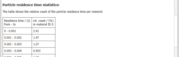
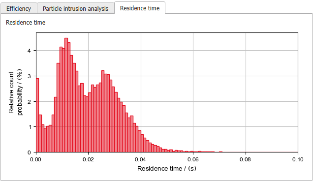
The Particle residence time statistics table shows how long a particle stays inside of a medium. For filter media simulations, particles can only reside inside of the fluid, which by default has material ID 0. So therefore, this table shows how long the particles moved inside of the fluid until they either deposited on the filter material or left the simulation area through the outlet.

The Residence time is subdivided into steps whose size is defined by the Max. time reached entered in the Filter Experiment tab divided by 1000.  

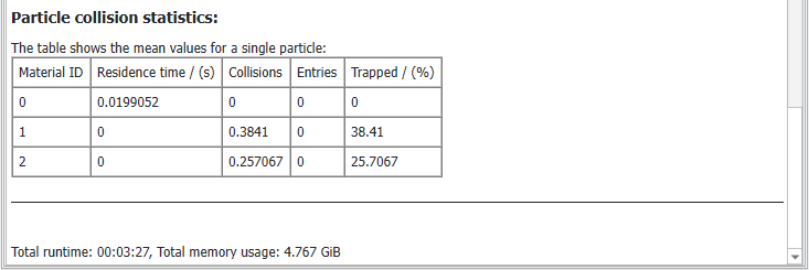
The Particle collision statistics table shows the mean value of the residence times in each material. In solid materials that the particle cannot enter, the residence time is 0. The Entries column shows how often particles enter into the corresponding material. In the above case, where material ID 0 is the fluid material, and material ID 1 and 2 are solid materials that the particles cannot enter, the number of entries is 0. The Trapped column shows the percentage of particles deposited on the surface of the material. The Collisions column shows the average number of collisions a particle has with the material surface. With the Caught On First Touch collision model, the number of collisions corresponds to the percentage of trapped particles, because every collision leads to a trapped particle.

Plots

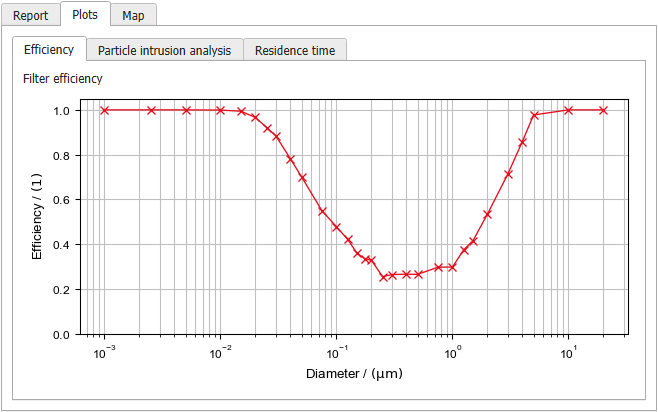
On the Plots tab, three sub-tabs are available. The Efficiency tab depicts the computed fractional filtration efficiencies:

Two plots are shown on the Particle Intrusion Analysis plot. The Cumulative Intrusion Depth shows for each particle type (i.e. particle size), how far particles of this size move into the filter before they are captured. Starting on the left, at Depth 0 still 100% of the particles are unfiltered. When moving into the filter, the percentage of unfiltered particles goes down, until at the downstream side the particles reach the outflow.

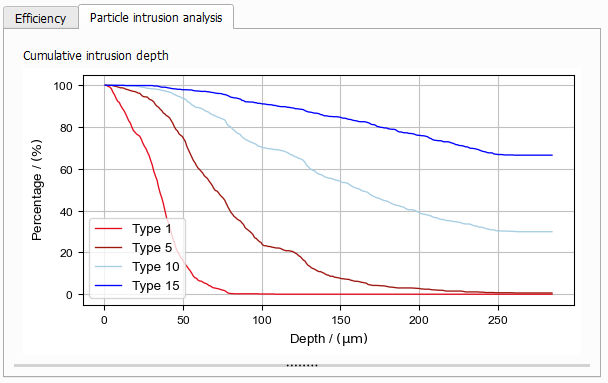
Right-click into the plot area to open a dialog box that lets you select which graphs are shown. For each particle type, you can additionally select to plot the fitted exponential decay function:

If the filter material is homogeneous over the depth of the filter, the probability that a moving particle hits a fiber is constant during the movement through the filter. In that case, the particle intrusion depth should follow an exponential decay, e.g. 50% are captured after the first 50 µm, 75% after 100 µm, 87.5% after 150 µm and so on. Therefore it is sensible to fit an exponential decay function through the computed intrusion depths as a model for the filter efficiency. The reported Depth Efficiency is the filtration efficiency predicted by this model.

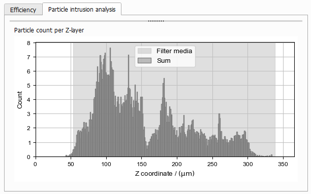
On the Particle count per Z-layer plot, the distribution of the collected particles over the filter height is plotted. For each particle type, the number of particles deposited on each Z-layer is counted. To reflect the given particles size distribution, this value is scaled with the particle types Count Percentage (recall that for Filter Efficiency simulations the same number of particles is simulated for each particle type independently of the given physical particles size distribution).

The Residence time plot plots the values shown in the Particle residence time statistics table.