|
Navigation: GeoDict 2026 - User Guide > Simulation & Prediction > FlowDict > Darcy Flow > Options > Solver |
Scroll |
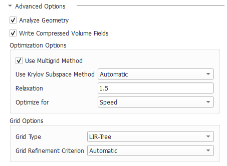
Advanced Options
Unfold Advanced Options to gain access to several advanced solver options.
Advanced Options for EJ:
Checking Analyze Geometry performs an analysis of the geometry before the solver computations.  If no percolation path through the structure is found, the partial differential equation does not need to be solved, and a permeability of 0.0 is directly reported as the solution. Furthermore, the solver operates on the whole structure, regardless of which parts are connected or unconnected. However, unconnected components are not transport relevant, thus the effort of solving in these parts is not necessary. For these reasons, a geometrical analysis is routinely run to determine whether a through path exists. After the analysis is finished, unconnected components are removed from the computational grid. This may speed up the computations but requires some time for the geometrical analysis, especially for very large structures. So if you know beforehand that there are no unrelevant parts or that the structure has been processed to eliminate them, the geometry analysis can be switched off by unchecking Analyze Geometry. |
Advanced Options for LIR:
Checking Analyze Geometry performs an analysis of the geometry before the solver computations. If no percolation path through the structure is found, the partial differential equation does not need to be solved, and a permeability of 0.0 is directly reported as the solution. Furthermore, the solver operates on the whole structure, regardless of which parts are connected or unconnected. However, unconnected components are not transport relevant, thus the effort of solving in these parts is not necessary. For these reasons, a geometrical analysis is routinely run to determine whether a through path exists. After the analysis is finished, unconnected components are removed from the computational grid. This may speed up the computations but requires some time for the geometrical analysis, especially for very large structures. So if you know beforehand that there are no unrelevant parts or that the structure has been processed to eliminate them, the geometry analysis can be switched off by unchecking Analyze Geometry. |
 Write Compressed Volume Fields
The LIR solver uses a very memory efficient adaptive grid structure for the simulations. If the option Write Compressed Volume Fields is checked, then the adaptive grid is used as compression method for writing out *.hht files. This option allows to save 80-90% space on hard drive. The runtime for writing *.hht files is also reduced significantly. But the runtime for loading and uncompressing of compressed *.hht is increased by the amount of runtime that was saved for writing out compressed *.hht files. If the option Write Compressed Volume Fields is not checked, then a usual regular grid is used for writing out *.hht files. |
The Multigrid Method (see e.g. Wesseling, 2004) was introduced to speed-up the computation and reduce the runtime significantly. The main idea of Multigrid is the usage of multiple coarser adaptive grids to speed up convergence behavior but requires only little more memory. The method is available to solve the Stokes and Stokes–Brinkman equations as well as for solving mechanics, diffusion, thermal, and electrical conduction and is enabled by default. Another speed-up option to accelerate the convergence behavior of the LIR solver is called Krylov Subspace Method. The runtime of the LIR solver depends on many different properties of the structure and the simulation parameters. The BiCGStab algorithm is used, which can reduce the runtime for challenging simulation very drastically.
Unfortunately, the Krylov method is not always faster than a simulation without the Krylov method and therefore we introduced an Automatic mode which uses some heuristics to choose the most efficient method based on structure, material parameters, and boundary conditions automatically. Of course, it is possible to explicitly enable (Enabled) or disable (Disabled) the method.
Depending on the material parameters and geometry of the structure, the underlying mathematical problem can vary in complexity, thus influencing the behavior of the solver. The more complex the problem is, the more stable the solver settings should be. With the Relaxation number, the solver is adjusted from Stable (which results in higher number of iterations, slower time stepping, and longer solver run times), to Fast, which makes the solver run less iterations but implies the risk that the solver does not converge. The Relaxation is a parameter of the SOR method and must be between 0 and 2 to ensure convergence. For relaxation values smaller than one (<1.0), the simulation is more stable. For relaxation values larger than one (>1.0), the simulation converges faster. The LIR solver can Optimize for Speed or Memory.
|

The Grid Type decides what kind of tree structure is used for the simulation. The default option is LIR-Tree and should always be used. The solver uses an adaptive grid structure called LIR-tree and needs up to 10 times less runtime and memory compared to the Regular Grid option. The solver can analyze the result field during the computation and improves the adaptive grid in places where more accuracy is needed. The LIR solver splits cells where a high gradient occurs. The solver refines the adaptive grid based on the computed fields. New cells are introduced at locations where higher accuracy is needed. Three settings are available here:
|

©2025 created by Math2Market GmbH / Imprint / Privacy Policy