Click OK to input the entered parameters, and then click Run in the FilterDict section to start the Filter Lifetime command. The results are immediately shown in the opening Result Viewer after the simulation is finished.
Report
Stopping Criterion
At the top of the Report, the stopping criteria reached by the simulation is shown. Here, it is also reported if the simulation was canceled (Stopped by user). If you open the result file while the simulation is still running, the first line reads Simulation unfinished.
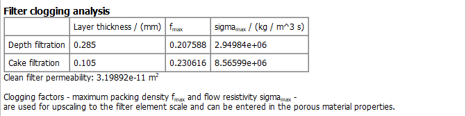
Filter Clogging Analysis
Below, the Filter clogging analysis analyzes the properties of the filter cake. These parameters can be used as input for simulations of filter elements or complete filters where it is not possible to resolve filter media and particles and an effective description of the filtration parameters is required.
The Depth filtration parameters are computed as follows:
The Layer thickness is the thickness of the filter media. All voxel layers containing solid voxels are considered as part of the filter media. Note, that this definition is different from the definition of the thickness used in the MatDict - Material Statistics – Thickness Estimation command.
is the maximum solid density achieved in one z-layer.
The flow resistivity caused by particles filtered in the depth of the filter media is computed as quotient of the pressure drop increase over the filter media (here, the same part is considered as for the Layer Thickness) and the average flow velocity :
(274)
This resistivity represents the average over all z-layers of the filter media, which does not directly correspond to the maximum solid density , but to the average solid density of all layers. is then computed by scaling the resistivity:
(275)
The Cake filtration parameters are computed if a sufficiently thick filter cake has formed. They are determined as follows:
All voxel layers in the inflow region which are at least partially filled with deposited dust are analyzed. is the maximum solid density achieved in a single z-layer in the inflow region.
The Layer thickness is the thickness of the filter cake. Here, only layers that achieve a solid volume fraction of at least 80% of are taken into account. Thus, dendrites forming on top of the cake are not taken into account when determining the thickness.
is flow resistivity, computed as quotient of the pressure drop over the filter cake (here, the same part is considered as for the Layer Thickness) and the average flow velocity.
The Clean filter permeability is the computed permeability of the clean filter. The value is computed using the Depth filtration - Layer thickness as thickness of the filter media.
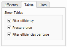
Tables
Below, a number of tables are presented, that can be selected under the Tables tab in the post-processing section on the left.
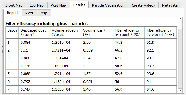
The Filter efficiency table contains, for every batch, the Deposited dust, the Volume added to the material by the deposited particles, the Volume loss, and the Filter efficiency in percentage by count and by weight.
For the computation of the efficiency, Efficiency results with ghost particles, controls how the results with and without ghost particles are displayed in the tables. Selecting Excluded and (Included), the tables contain the efficiency without ghost particles and additionally the efficiency with ghost particles in brackets. The other two options, Excluded or Included, show either the result with or without ghost particles. This option is only available if the user selected to run the simulation with ghost particles.
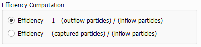
The Efficiency Computation panel allows to select the definition of the filtration efficiency. It can either be based on the number of particles which leave the domain via the outflow region or on the number of particles which are captured. The difference between both definitions is the handling of particles which are still in the domain but are not (yet) marked as captured.
The Volume loss is the particle volume lost during each batch due to the overlapping of particles. This value is a good indicator whether the number of particles per batch has been chosen correctly. If the Volume Loss is too high, the number of particles per batch should be reduced to achieve a sufficient accuracy of the computation.
The overall volume loss is reported below the Filter Efficiency table:
For simulation with Unresolved particles, also the number of voxels filled by a higher volume fraction than the defined maximal packing density is reported. If some particles are smaller and some are larger than the voxel length, the number of overpacked voxels is typically very large (all locations where a large particle is deposited are overpacked, because a large particle fills up several voxels completely).
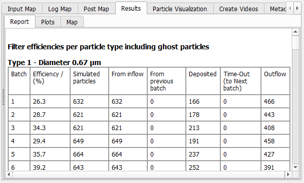
The Filter efficiencies per particle type tables show the filter Efficiency of a certain particle type for every batch. It shows the overall number of Simulated particles, consisting of particles entering Frominflow, or continuing movement From previous batch. At the end of the batch, particles are either Deposited, are still moving inside of the structure (Time-Out), or have left the domain through the Outflow.
Depending on the choice of input parameters, some particles may neither count as Deposited, Time-Out or Outflow, e.g. because they leave the domain through the inflow area. In this case, those particles are removed completely from the reported statistics Those particles are not included in the number of Simulated Particles.
If in a batch the number of Simulated Particles of one particle type (diameter) is 0, the efficiency of this particle type cannot be computed from the statistics (0/0 particles are filtered). In that case, the efficiency of this type is set to the efficiency of the next particle type (next larger diameter). If no particle with a larger diameter exists, the efficiency is assumed to be 100%. Use Ghost Particles to assure that a sufficiently large number of particles of each type is simulated in every batch.
Plots
The Plots tab always shows the two plots Pressure drop over time and Deposited dust over time. You can select additional plots in the Plots tab in the post-processing section on the left hand side. Simply select the plots to be created and click the Apply button.
The plots appear sorted into sub-tabs in the Plots area on the right hand side. Up to two plots are shown above each other. If more plots are generated, a dropdown-menu allows to select the plot to be shown. The following plots are available
The Pressure drop over time and Deposited dust over time are always shown in the Lifetime results tab. Pressure drop over deposited dust and Pressure drop over challenge dust appear additionally if selected.
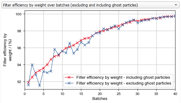
You can plot the filter efficiency development over the computed batches, either computed by weight or by count. Efficiency by count is typically dominated by the small particles, whereas Efficiency by weight mostly depends on the large particles.
The plots respect the choices made on the Efficiency tab regarding the computation of the efficiency and the inclusion of ghost particles. If you select Excluded and Included for the ghost particles, you can see the graphs for both options and compare the results.
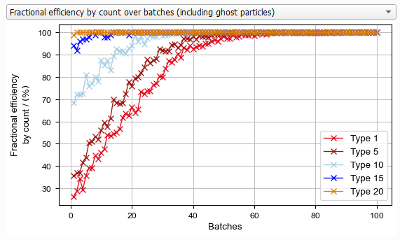
The Fractional efficiency over batches plot shows the evolution of the fractional filter efficiency over time. For each particle type, an individual efficiency curve is plotted.
The Efficiency over particle type for first XX batches plot shows the fractional efficiencies plotted over the particle sizes on the x-axis. The plot shows the curves for each of the batches and also the mean over the selected range.
Two plots are shown on the Particle Intrusion Analysis plot. The Cumulative Intrusion Depth shows for each particle type (i.e. particle size), how far particles of this size move into the filter before they are captured. Starting on the left, at Depth 0 still 100% of the particles are unfiltered. When moving into the filter, the percentage of unfiltered particles goes down, until at the downstream side the particles reach the outflow.
Important! The plot only takes the results of the first batch into account when the filter is still clean.
Right-click into the plot area to open a dialog box that lets you select which graphs are shown. For each particle type, you can additionally select to plot the fitted exponential decay function:
If the filter material is homogeneous over the depth of the filter, the probability that a moving particle hits a fiber is constant during the movement through the filter. In that case, the particle intrusion depth should follow an exponential decay, e.g. 50% are captured after the first 50 µm, 75% after 100 µm, 87.5% after 150 µm and so on. Therefore it is sensible to fit an exponential decay function through the computed intrusion depths as a model for the filter efficiency. The reported Depth Efficiency is the filtration efficiency predicted by this model.
On the Particle count per Z-layer plot, the distribution of the collected particles over the filter height is plotted. For each particle type, the number of particles deposited on each Z-layer is counted.
Only the results of the first batch are included in this graph, too. Ghost particles are not taken into account. Be aware that the x-axis of the Particle count per Z-layer plot includes inflow and outflow area, while the x-axis of the Cumulative intrusion depth plot shows only the filter media (the range marked in gray in the lower plot).
These plots show the average pressure per voxel layer in the structure for every time step. A steep increase in a certain layer indicates that the filter is blocked in that layer.
Select the time step with the Layered pressure: Time step pull-down menu.
The Convergence tab displays the convergence of the flow solver over the iterations for every time step (which was also shown in the progress dialog while the solver was running). The convergence chart can be a tool to check if the flow solver parameters were chosen correctly.
 Filter efficiency