This folder contains the original structure model on which the identification was done (Structure.gdt) and the resulting structure with identified target material (labeledStructure.gdt). Also, the neural network output file (nnOutput.npz) is saved in the folder and can be reused as described here.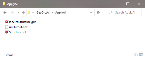

The GeoDict Result Viewer opens for the result file. In the Report for two-channel analysis the solid volume percentage of the labeled target material is given.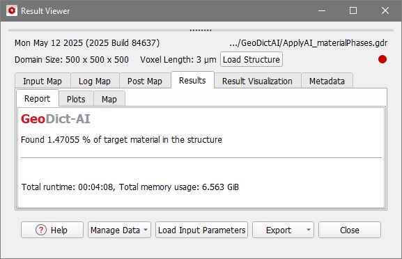

In the Result Viewer, under the Results - Plots subtab, for two-channel analysis find the solid volume percentage distribution of the target material per slice in Z-direction.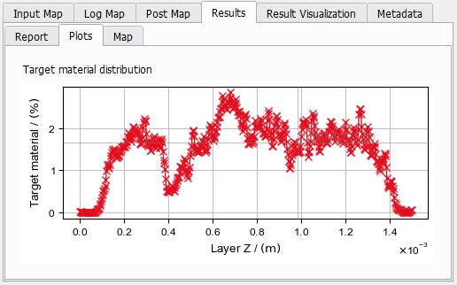

To visualize the target material identified by the network, move to the Result Visualization tab. There, click Load *.gdt for Load Structure with Labels.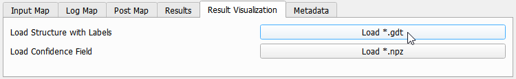

The identified target materials are assigned to the next free materials IDs, and thus, are shown in the colors selected for these IDs.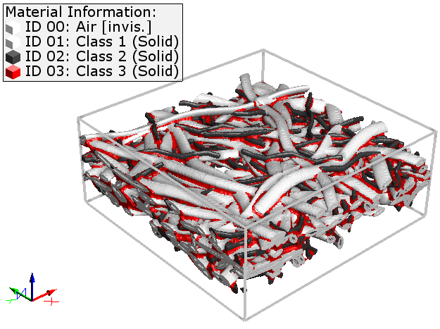

Click the Load *.npz button next to Load Confidence Field to load the unassigned data of the material identification. The analyzed material is split into the materials the network was trained for. For example, consider a neural network trained to distinguish the solid material into cellulose fibers (channel 0), ellipsoidal fibers (channel 1) and binder (channel 2). Then each of them gets their own material ID after applying the network. For each channel a confidence field is created.

Set the structure to invisible, by unchecking the Structure tab in the View Controls, above the Visualization area. Move to the Volume Field tab to control the visualization of the confidence field. Deselect the IDs for Visible on Material IDs to only see the values of interest. In the example the confidence field for channel 1 (ellipsoidal fibers) is shown. The red voxels mean that the network was very confident that these voxels belong to channel one and  blue means, it is very confident that these voxels do not belong to circular fibers. Most voxels are either red or blue. Thus, the network was overall very confident with it's result.

To show the voxels where the network was less confident you can use the confidence value as described here. In the following example the value was set to 0.9. Thus, all voxels assigned to ID 255 have a confidence value smaller than 0.9 for all three channels. For all other voxels the material is chosen depending on which channel has the highest confidence value.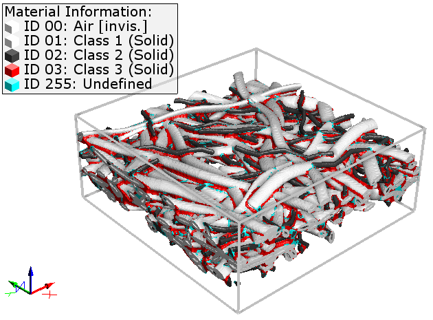

You can also threshold the confidence field in the visualization area depending on the confidence value. For two-channel models, this is useful to visualize the Threshold for the Target Material. For this, visualize the numpy field for channel 1 and change the clipping value to separate the values for the different materials. If the Threshold was set to 0.5, entering 0.5 for the volume field threshold and selecting >= as clip mode visualizes only the result values for the identified target material. For a well-performing network most of the values in the volume field should be near 1 (target material) or near 0 (original material), meaning the network is confident with the classification for the corresponding voxel. This can be observed in the example below. After clipping away all voxels with a value smaller than 0.5, most of the remaining voxels are red, i.e. near 1.

For more visualization options refer to the Visualization handbook.