The AcoustoDict Johnson–Champoux–Allard Model Options dialog opens when clicking the Options’ Edit… button in the AcoustoDict section.
The options necessary to run the solvers can be entered under the Constituent Materials, Boundary Conditions, Flow Solver, and DiffusionSolver tabs. The command internally has to solve two partial differential equations:
The Stokes equations to compute the air flow resistivity,
The Laplace equation to determine the tortuosity.
The Equations and References tab displays further information about the model.
Constituent Materials
Under the Constituent Materials tab, all parameters are as described for the Delany–Bazley model. The Allard–Johnson model also assumes that the fluid in the pore space is air and it should be set that way.
Boundary Conditions
For the Boundary Conditions, the options are the same as for the Delany–Bazley model.
Flow Solver
The parameters entered under the Flow Solver tab have the same meaning as described for the Delany–Bazley model.
Diffusion Solver
AcoustoDict solves the Laplace equation to compute tortuosity, diffusivity, and viscous characteristic length. For this, the EJ solver is used.
The equations are solved by an iterative approach.
Iterative Solver
The basic idea of an iterative method is to
Start with some initial guess for the unknown values
Improve the current values in each iterative step
Repeat the iterative process until one of the stopping criteria is reached.
The iterative process is controlled by setting the values and activation for Tolerance, Residual, Maximal Iterations, and Maximal Run Time (h). The stopping criteria apply for each computational direction individually.
If multiple stopping criteria are selected, the first criterion that is reached causes the solver to stop.
The Tolerance stopping criterion, the default stopping criterion for EJ, looks for stagnation of the method when the process becomes stationary, i.e. the improvement in the permeability value becomes extremely small from iteration to iteration.
In each iteration, the solver checks for the current computed value against the values of the last 100 iterations if there are any changes.
(88)
The computation is stopped if the maximal relative change is smaller than the value entered for Tolerance. When there is doubt about the quality of the solution, decrease the Tolerance value by a factor of ten. The drawback of this criterion is that the solver sometimes might stop too early in case of slow convergence rate or at local extrema of oscillatory convergence curves.
When the Residual stopping criterion is used, the iteration is stopped if the solution satisfies the equation up to the required accuracy.
By setting the stopping criterion to Residual, the computations terminate as soon as the relative norm drops below the selected residual threshold. The relative norm of the Schur Complement residual is computed and displayed in the console window during the calculations. The console is visible by clicking the double arrow button on the lower right corner in the progress dialog.
The recommendation to choose Tolerance or Residual for the EJ solver is based on the structure’s porosity. Both give similar results for highly porous structures. For dense structures, if using the Schur Complement Residual, the relative norm of the residual may be small even though the correct permeability has not been reached. So, when in doubt, use the Tolerance criteria – the default option.
Use the Maximum Iterations value or the Maximum Run Time (h) stopping criteria causes the solver to stop if the maximal number of iterations and/or the maximal run time (in hours) is exceeded.
When the solver stops because one of these criteria has been reached, no guarantee on the quality of solution can be given. In this case, a warning is printed into the report. The following possibilities might help:
Check the corresponding .log file to see how large the residual values and permeability values are. If permeability values are in reasonable range and they do not have changed during the last iterations, you may decide to use the current result.
Double-check the structure and parameter values. Unphysical parameters or too rough resolution of the structure (leading, e.g., to artificial unconnected components) can cause an iterative solver to fail.
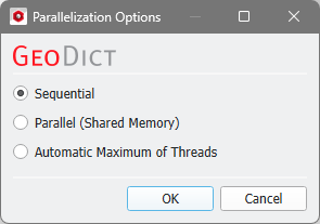
Control how many threads are used for the computation. Parallelization is possible if your license and hardware allow it.
The Parallelization Options dialog opens when clicking the Edit button and you can choose between Sequential, Parallel (Shared Memory), or Automatic Maximum of Threads.
Selecting Sequential will not apply parallelization and only one thread is used for the computation.
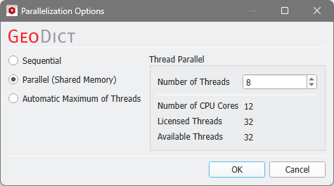
When Parallel (Shared Memory) is selected, the Number of Threads can be entered. Below, the Number of CPU Cores that the current machine has, the maximum number of Licensed Threads and the number of those licensed threads that are available (Available Threads) are shown in the dialog. Of course, the maximal number of parallel processes you can use, is the smallest of those three numbers.
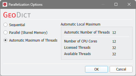
If Automatic Maximum of Threads is selected, the number of parallel processes is automatically selected for optimal speed, based on the CPU cores and licensed parallel processes.
The Automatic Local Maximum of processes is automatically selected, which is the minimum of Number of CPU Cores, Licensed Threads, and Available Threads.
Additionally, for the EJ solver, calculations can run on a Linux cluster.
For more details on how to set up and run parallel computations, consult the High Performance Computing chapter.
Checking Discard PDE Solver Files causes the deletion of all intermediate computation files, such as log files and flow field files.
Only the content of the final GeoDict result file (*.gdr) is stored.
While having the benefit of saving hard disk storage place, discarding intermediate solver files has also the effect of disabling the 3D visualization of the results.
Additional 3D data can be added to the solution *.hht files for visualization or later analysis. With Write Diffusion Flux into Solution File the Diffusion Flux in the three coordinate directions is saved, allowing a detailed analysis of the field. The size of the result files and the memory requirements increase when selecting this option.
Equations and References
This tab displays formulas and references which are explained in more detail in the Theoretical Background.


 Write Diffusion Flux into Solution File