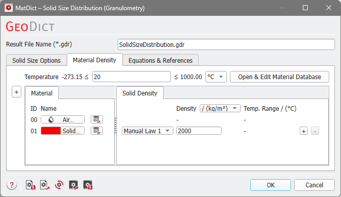
The Solid Size Distribution dialog includes the Solid Size Options and the Material Density tabs. The last tab, Equations & References, provides further information about the underlying algorithm and cites J. Becker, A.Wiegmann, T. Saito, and D. Silin.
At the top of the dialog, enter the Result File Name. The result file is saved in the chosen project folder (File → Choose Project Folder in the menu bar).
Enter the Bin Size in units of voxels. The equivalent in metric length units is shown on the right. The bin size determines the range of diameters that belong to one class of solid sizes.
All bins have equal bin size. Beginning with the largest possible diameter that is divisible by the bin size, the diameter is reduced by the bin size in each step. Every voxel is then assigned the diameter of the largest possible sphere that can be fitted in the solid and contains this voxel. Thus, each bin contains solid voxels with an assigned diameter in the range comprised between and , where is the bin number.
For example, when analyzing a porous structure with a voxel size of 1 µm, you can set the bin size to 2 or to 4 (voxels) which would come to classify the solid by their diameter in ranges of 2 µm or 4 µm, and would result in the following bins:
Bin number ()
Pore diameter between
Bin Size 2 µm
Bin Size 4 µm
1
0 µm - 2 µm
0 µm - 4 µm
2
2 µm - 4 µm
4 µm - 8 µm
3
4 µm - 6 µm
8 µm - 12 µm
..
...
...
When choosing the bin size, be aware that the underlying algorithm to compute the Euclidean distance operates directly on the voxel grid. Thus, the smallest possible distance between two grid points is 1 voxel, which corresponds to a radius of 1 voxel. This means the smallest diameter that the algorithm will find is 2 voxels. In general, the error made when computing the solid size distribution is of the same order of magnitude as the discretization error of the structure, i.e., 1 voxel.
In the result viewer, for each bin the Minimal Diameter, which is the diameter of the smaller sphere, and the Maximal Diameter, which is the diameter of the larger sphere, are given. This means all solid voxels in that bin have a diameter that is larger than the minimal diameter and smaller or equal than the maximal diameter.
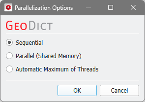
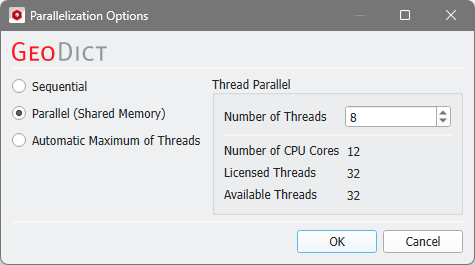
Control how many threads are used for the computation. Parallelization is possible if your license and hardware allow it.
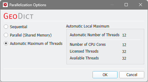
The Parallelization Options dialog opens when clicking the Edit button and you can choose between Sequential, Parallel (Shared Memory), or Automatic Maximum of Threads.
Selecting Sequential will not apply parallelization and only one thread is used for the computation.
When Parallel (Shared Memory) is selected, the Number of Threads can be entered. Below, the Number of CPU Cores that the current machine has, the maximum number of Licensed Threads and the number of those licensed threads that are available (Available Threads) are shown in the dialog. Of course, the maximal number of parallel processes you can use, is the smallest of those three numbers.
If Automatic Maximum of Threads is selected, the number of parallel processes is automatically selected for optimal speed, based on the CPU cores and licensed parallel processes.
The Automatic Local Maximum of processes is automatically selected, which is the minimum of Number of CPU Cores, Licensed Threads, and Available Threads.
The Domain Boundary Conditions can be chosen to be Symmetric, Periodic, Encase, or any combinations of those boundary conditions in all three directions with the choice of Expert.
Choosing the appropriate boundary condition depends on the structure’s design.
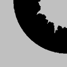
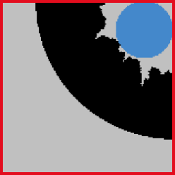
For example, imagine a structure with a cross-section as shown below.
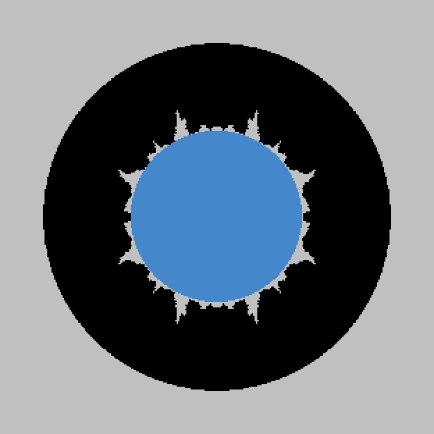
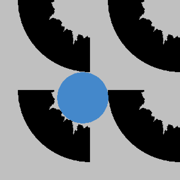
For the three boundary condition options the resulting solid size is visualized in blue.
If Symmetric boundary conditions are taken, the geometry is mirrored at the domain boundary.
If instead the expected pattern of the geometry is repeated in all directions, Periodic boundary conditions should be selected. That has the effect that the objects and pores of the structure that end on one side of the structure reappear on the opposite side.
If the structure should be encased with a closed wall, the Encase boundary conditions are used.
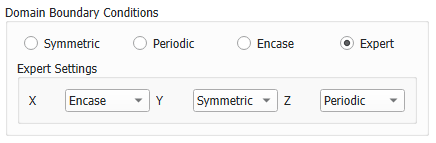
Check Expert to apply different boundary conditions for each direction. You can combine the three above mentioned boundary conditions independently for the directions. For example, the boundary conditions could be chosen to be Encase in X-direction, Symmetric in the Y-direction and Periodic in Z-direction.
When Write Solid Size Distribution as *.gsd File is checked, a file with the default name SolidSizeDistribution.gsd, in *.gsd (GeoDict Size Distribution) format, is saved in the results folder inside the project folder. The file contains the solid size (diameter of sphere) of each voxel written into a volume field that can be loaded in the Solid Size Visualization tab of the Result Viewer.
Material Density
Under the Material Density tab, the temperature can be edited if the density of a material is temperature dependent. Additionally, the density of every solid material in the structure must be specified in this tab. The density can be given in kg/m3 or g/cm3. For materials from the GeoDict Material Database, the density value is entered automatically. If a material is set to Manual, the Material Law changes to Manual Law and more laws can be added or deleted by clicking the “+” or “-“ button on the right of the corresponding row. You can enter the density for manual materials directly in this tab.


 Write Solid Size Distribution as *.gsd File