The Solver tab contains on the left the Flow Calculation, Batch Settings and the Parallelization setup and on the right individual tabs for every solver. Tabs corresponding to unused solvers are grayed out and not selectable.

Flow Calculation

FilterDict treats the flow for the first (initial) batch and all subsequent (iterative) batches differently for two main reasons:

• In the initial batch, the filter is still clean, while in all iterative batches, previously deposited particles are present.
• In all iterative steps, the flow solver can use the solution of the previous step as initial guess, which is not possible for the initial batch.

The names of the equations to solve the Initial Flow PDE and Iterative Flow PDE are shown for information. These entries cannot be changed directly because they depend on the selection of Resolved / Unresolved particles in the Constituent Materials tab and the choice of Creeping / Fast Flow in Flow Motion under the Filter Experiment tab.

To solve the Flow PDEs, different flow solvers are available as Initial Flow Solver and as Iterative Flow Solver (SimpleFFT or LIR). The initial flow field may alternatively also be loaded from a previous FilterDict or FlowDict computation.

Tooltips help choosing the appropriate Initial and Iterative Flow Solvers. The default choice is the LIR solver for both the initial and the iterative flow solver. In most cases, LIR is computationally more efficient than SimpleFFT.

Analyze Geometry

If this option is chosen, a geometrical analysis at first determines whether a through path exists and removes unconnected pore components from the computational grid. This may speed up the flow computations but requires time for the geometrical analysis.

Batch Settings

The number of Batches per Flow Field determines how often the flow field is re-computed. Usually, the flow field should be recomputed for every batch (time interval), but if this is numerically too costly, it can be changed to re-compute the flow field only after every second or third batch. However, when more than one batch per flow field is chosen, the accuracy of the result decreases. In this case, numerical artifacts might be introduced. The most accurate results are obtained by computing one batch per flow field.

A batch of particles corresponds to a certain time interval in the experiment. The particles simulated in a batch do not interact with each other, but they do interact with the particles deposited in the previous batches. Decreasing the number of particles per batch leads to a higher accuracy, but also to longer simulation times.

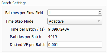
The length of the time intervals per batch and the number of particles can be chosen by selecting a Time Step Mode from the pull-down menu:

Adaptive

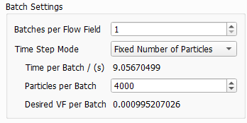
Fixed Number of Particles

Fixed Time

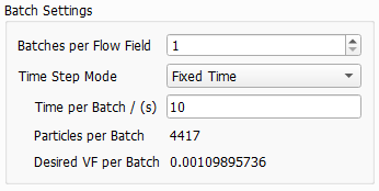
For multi pass simulations, Fixed Number or Adaptive should be preferred over Fixed Time. The particle concentration in the fluid changes over time. Therefore, also the number of particles could change significantly with Fixed Time steps and this might lead to a less stable simulation.

Parallelization

Depending on the purchased license, the simulation process can be parallelized. The Parallelization Options dialog opens when clicking the Edit... button, to choose between Sequential, Parallel (Shared Memory), Automatic Number of Threads and Cluster. For details on how to set up und run parallel computations, refer to the High Performance Computations handbook

The chosen parallelization settings apply for all steps of the simulation. Per default, the Automatic Number of Threads option is used, and the exact number of threads depends on the number of cores on the current computer and the number of licensed processes.

Load

How to load a previously computed flow field is explained here.

SimpleFFT and LIR

The settings for the chosen solver are explained in detail in the FlowDict handbook.