Solver
The Solver tab contains on the left the Flow Calculation, Batch Settings and the Parallelization setup and on the right individual tabs for every solver. Tabs corresponding to unused solvers are grayed out and not selectable.
Flow Calculation
FilterDict treats the flow for the first (initial) batch and all subsequent (iterative) batches differently for two main reasons:
- In the initial batch, the filter is still clean, while in all iterative batches, previously deposited particles are present.
- In all iterative steps, the flow solver can use the solution of the previous step as initial guess, which is not possible for the initial batch.
The names of the equations to solve the Initial Flow PDE and Iterative Flow PDE are shown for information. These entries cannot be changed directly because they depend on the selection of Resolved / Unresolved particles in the Constituent Materials tab and the choice of Creeping / Fast Flow in Flow Motion under the Filter Experiment tab.
To solve the Flow PDEs, different flow solvers are available as Initial Flow Solver and as Iterative Flow Solver (EJ, SimpleFFT or LIR). The initial flow field may alternatively also be loaded from a previous FilterDict or FlowDict computation.
Tooltips help choosing the appropriate Initial and Iterative Flow Solvers. The default choice is the LIR solver for both the initial and the iterative flow solver. In most cases, LIR is computationally more efficient than EJ or SimpleFFT.
Analyze Geometry
If this option is chosen, a geometrical analysis at first determines whether a through path exists and removes unconnected pore components from the computational grid. This may speed up the flow computations but requires time for the geometrical analysis.
Batch Settings
The number of Batches per Flow Field determines how often the flow field is re-computed. Usually, the flow field should be recomputed for every batch (time interval), but if this is numerically too costly, it can be changed to re-compute the flow field only after every second or third batch. However, when more than one batch per flow field is chosen, the accuracy of the result decreases. In this case, numerical artifacts might be introduced. The most accurate results are obtained by computing one batch per flow field.
A batch of particles corresponds to a certain time interval in the experiment. The particles simulated in a batch do not interact with each other, but they do interact with the particles deposited in the previous batches. Decreasing the number of particles per batch leads to a higher accuracy, but also to longer simulation times.
The length of the time intervals per batch and the number of particles can be chosen by selecting a Time Step Mode from the pull-down menu:
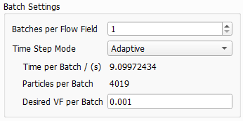
 Fixed Number of Particles
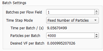
Fixed Time
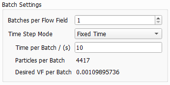
For multi pass simulations, Fixed Number or Adaptive should be preferred over Fixed Time. The particle concentration in the fluid changes over time. Therefore, also the number of particles could change significantly with Fixed Time steps and this might lead to a less stable simulation.
Parallelization
Depending on the purchased license, the simulation process can be parallelized. The Parallelization Options dialog opens when clicking the Edit... button, to choose between Sequential, Parallel (Shared Memory), Automatic Number of Threads and Cluster. For details on how to set up und run parallel computations, refer to the High Performance Computations handbook
The chosen parallelization settings apply for all steps of the simulation. Per default, the Automatic Number of Threads option is used, and the exact number of threads depends on the number of cores on the current computer and the number of licensed processes.
|
Parallelization Benchmark Results The example computation was run on a server with 2xIntel E5-2697A v4 processors with 16 cores each, running with a maximum of 3.60GHz. The input structure is an air filter media of size 1024x1024x768 voxels. A filter lifetime single pass simulation was run for a particle distribution according to ISO A1 ultrafine particles. 50 batches were computed with a time per batch of 10 s. For each batch approximately 35000 particles were simulated. The flow was computed with the LIR solver, which required approx 30 GB of RAm to run the simulation. The plot shows the runtime for a different number of processes for the whole simulation. The ideal speedup, i.e. getting half the runtime for twice the number of processes, is also shown as a gray dashed line. For the computation of 50 batches, a significant part of the runtime is spent for input and output in this example, as is typical for filter simulations. This leads to a reduced speedup when using a large number of processes for a small sized structure size. |

Load
With Load from File, a flow field from a previously run flow simulation is used. The flow field may originate from a FlowDict simulation or from a FilterDict simulation.
When calculated with FlowDict, the user needs to make sure to:
- Add inflow and outflow regions to the media model before running FilterDict.
- Compute the flow in the Z-direction
- Set the accuracy at least one order of magnitude higher than the default in FlowDict (e.g., Error Bound = 0.001 instead of 0.01). The stopping criteria depend on global values, whereas the particle movement depends on the local flow field which is subjected to larger deviations.
As mentioned above, depending on the velocity of the flow, the user may have decided to solve the Stokes or the Navier-Stokes equations with the flow solvers when running the simulation (that will be loaded now) in FlowDict.
Under the Load tab, click Browse and choose a flow field result file (GDR) to open. If no flow field is selected, a warning message appears (No flow field chosen) when trying to run the simulation.
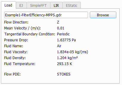
The physical properties of the fluid used in the flow simulation are entered automatically when loading the flow GDR file and appear listed under the Load tab.
- The Flow direction: Z is the main direction of the flow.
- The Mean Velocity of the flow field, the used Tangential Boundary Conditions and the Pressure Drop are taken from the loaded flow simulation. If the flow result was obtained by solving the Stokes equation, the solution is linear and will be rescaled automatically to match the Mean Velocity entered in the Filter Experiment tab.
- The fluid parameters Fluid Viscosity, Fluid Density, and Fluid Temperature are the physical values of the fluid used by the solver for the calculation of the flow field.
The fluid settings chosen under the Constituent Materials must be the same as the fluid that was used in the previously run flow simulation, loaded through the GDR file. Also, the Tangential Boundary Conditions selected in the Filter Experiment tab must match with those used in the flow simulation.
EJ, SimpleFFT and LIR
The settings for the chosen solver are explained in detail in the FlowDict handbook.
Estatic
The EStatic tab is becomes editable when Include Electrostatic Effects has been checked on the Electrostatic Effects tab. Equation (247) is solved to calculate the electrostatic potential.
The Dirichlet Boundary Offset is the offset (in Voxels), where the zero Dirichlet boundary conditions for the potential apply. For large numbers , the computation is more accurate but also requires more numerical resources. This increment of the computational domain occurs internally for the electrostatic solver and does not influence the structure seen by the user in the visualization area.