In the Flow Calculation panel, select the flow solver used to compute the flow field or choose to load a flow field already precomputed in a previous computation. Depending on the Flow Motion type chosen on the Filter Experiment tab, either the Stokes or Navier-Stokes equations are solved. Three solvers EJ (only for Stokes flow), SimpleFFT and LIR are available.

Analyze Geometry

If this option is chosen, a geometrical analysis at first determines whether a through path exists and removes unconnected pore components from the computational grid. This may speed up the flow computations but requires time for the geometrical analysis.

Parallelization

Depending on the purchased license, the simulation process can be parallelized. The Parallelization Options dialog opens when clicking the Edit... button, to choose between Sequential, Parallel (Shared Memory), Automatic Number of Threads and Cluster. For details on how to set up und run parallel computations, refer to the High Performance Computations handbook

The chosen parallelization settings apply for all steps of the simulation. Per default, the Automatic Number of Threads option is used, and the exact number of threads depends on the number of cores on the current computer and the number of licensed processes.

Load from File

Select Load From File in the Flow Calculation panel to use a precomputed flow field. The flow field may originate from a FlowDict simulation or from a FilterDict simulation. When calculated with FlowDict, you have to make sure to:

1. Add inflow and outflow regions to the media model before running FilterDict.
2. Compute the flow in the Z-direction. You may either use the Stokes or Navier-Stokes equations depending on the flow velocity for this.
3. Set the accuracy at least one order of magnitude higher than the default in FlowDict (e.g., Error Bound = 0.001 instead of 0.01). The stopping criteria depend on global values, whereas the particle movement depends on the local flow field which is subjected to larger deviations.

Under the Load tab, click Browse and choose a result file (GDR) to open. If no flow field is selected, a warning message appears (No flow field chosen) when trying to run the simulation.

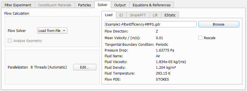
The physical properties of the fluid used in the flow simulation are entered automatically when loading the flow GDR file and appear listed under the Load tab.

• The Flow direction: Z is the main direction of the flow.
• The Mean Velocity [m/s] of the flow field, the used Tangential Boundary Conditions and the Pressure Drop are taken from the loaded flow simulation. If the flow result was obtained by solving the Stokes equation, the solution is linear and can be rescaled. When checking Rescale, the value that was entered automatically from the flow result file can be manually changed. Changing the mean velocity automatically rescales the pressure drop, too.
• The fluid parameters Fluid Viscosity [Pas], Fluid Density [kg/m³], and Fluid Temperature [K] are the physical values of the fluid used by the solver for the calculation of the flow field.

The fluid settings must be the same as the fluid that was used in the previously run flow simulation, loaded through the GDR file. Therefore, the Constituent Materials tab is inactive when Load from File is selected. Also, the Tangential Boundary Conditions selected in the Filter Experiment tab must match with those used in the flow simulation.

EJ, SimpleFFT, and LIR

In FilterDict, different solvers are available for the computation of the flow field.

These options are explained in detail in the FlowDict handbook. Be aware that the default accuracy in FilterDict is one order of magnitude higher than in FlowDict (Error Bound, Tolerance and Residual). The stopping criteria depend on global values, whereas the particle movement depends on the local flow field. It is therefore necessary to make sure that not only the overall pressure drop is computed up to the given accuracy, but that also the local values are sufficiently accurate. This typically achieved by setting a higher accuracy as stopping criterion.

Estatic

The EStatic tab is becomes editable when Include Electrostatic Effects has been checked on the Electrostatic Effects tab. Equation (247) is solved to calculate the electrostatic potential.

The Dirichlet Boundary Offset is the offset (in Voxels), where the zero Dirichlet boundary conditions for the potential apply. For large numbers , the computation is more accurate but also requires more numerical resources. This increment of the computational domain occurs internally for the electrostatic solver and does not influence the structure seen by the user in the visualization area.