|
Navigation: GeoDict 2026 - User Guide > Simulation & Prediction > BatteryDict > Battery > Charge Battery > Options |
Scroll |
Solver
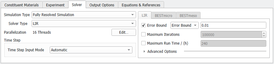
Under the Solver tab, select the type of simulation to run and the solver to use when solving the system of partial differential equations, as well as the solver options.

Select the Simulation Type to one of the following:
|
For a Fully Resolved Simulation, select LIR or BESTmicro for Solver Type. For the Homogenized Simulation, only the BESTmeso solver is available. If using any of the other two simulation types none of the solvers are used. For the LIR solver, additional parameters for the computation can be defined. |
Control how many threads are used for the computation. Parallelization is possible if your license and hardware allow it. The Parallelization Options dialog opens when clicking the Edit button and you can choose between Sequential, Parallel (Shared Memory), or Automatic Maximum of Threads.  Selecting Sequential will not apply parallelization and only one thread is used for the computation. 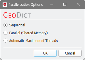 When Parallel (Shared Memory) is selected, the Number of Threads can be entered. Below, the Number of CPU Cores that the current machine has, the maximum number of Licensed Threads and the number of those licensed threads that are available (Available Threads) are shown in the dialog. Of course, the maximal number of parallel processes you can use, is the smallest of those three numbers. 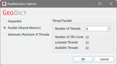 If Automatic Maximum of Threads is selected, the number of parallel processes is automatically selected for optimal speed, based on the CPU cores and licensed parallel processes. 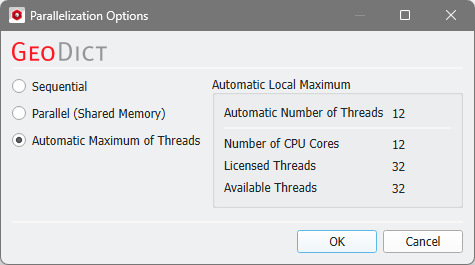 The Automatic Local Maximum of processes is automatically selected, which is the minimum of Number of CPU Cores, Licensed Threads, and Available Threads.
|

In the Time Step panel an option for the Time-Step Input Mode may be selected. Any of the battery solvers calculates the time evolution of the given Li-ion battery. It starts at the initial state, which has time = 0 in the result plots. It takes the time step defined as maximum time step size and tries to find the battery state at time = last time + time step by searching an equilibrium solution fulfilling the given system of differential equations. If no solution can be found for this time step size, it reduces the time step size, and the solver starts again. This procedure is repeated until an appropriate time step size is found. This time step size is used for the next steps in the simulation as well. After several successful steps with a certain time step size, the solver tries to increase this time step size again, to reduce overall computation time. With the Time-Step Input Mode, the maximum time-step size can be influenced. For more information on time steps see State of Charge (SOC) and State of Lithiation (SOL).
The time steps that were finally realized in the simulation are saved in the Result Map of the GeoDict result file (*.gdr file), created for the charging simulation, under the key TimeDependentValues:TimeStep. If a new battery state is found in a simulation with a charge rate boundary condition, the solver computes the Cell-SOC step of the just found new battery state i via: with the time step and the charge rate. So, it is not clear from the start which is the next computed Cell-SOC in a simulation, this depends on the time step. Example:
If you choose to set the current density instead of the charge rate, then the calculation of the Cell-SOC step size depends on the given current density and the cell capacity. Thereby, the cell capacity depends on the battery-geometry and the maximum lithium concentration of the active materials. In the GeoDict result file (*.gdr file) created for the charging simulation, you can find the time-evolution of the Cell-SOCs in percent as well as the corresponding times in seconds in the Result Map under the keys TimeDependentValues:CellStateOfCharge and TimeDependentValues:Time, respectively. For simple simulations (charge rate <= 1, physical domain size < = 5 µm, only one active material per electrode, diffusivities >= 1e-12 m²/s, conductivities >= 1 S/m and no warnings during the simulation), the time step size is usually the maximum time step size set. Then, also the Cell-SOC step is a constant value. However, for more complex simulations (charge rate >= 10, physical domain size >= 50 µm, two active materials in an electrode with different parameters, low diffusivities in the active materials and small conductivities), it might happen that the time step size may be smaller than the maximum time step size defined and not constant over the whole simulation. |
With the LIR solver, the partial differential equations of each time step are solved iteratively with an adaptive tree structure. Several solver options can be chosen in the panel on the right. 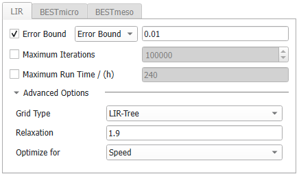 The stopping criterion Error Bound uses the result of previous iterations, and predicts the final solution based on linear and quadratic extrapolation. The solver stops if the relative difference between computed and predicted solution is smaller than the specified error bound. The stopping criterion recognizes oscillations in the convergence behavior and prevents premature stopping at local minima or maxima. A damped convergence curve is fit through the oscillating curve and the solver stops then regarding the damped convergence curve. If the Krylov method (under LIR - Advanced Options) is activated, which is always the case in BatteryDict, the definition of Error Bound is somewhat different. Here, no prediction is made, instead the continuity between neighboring cells and the conservation of mass is checked. The maximal value is normalized by the mean flow and if this value is smaller than the Error Bound the simulation stops. Use the Maximum Iterations value or the Maximum Run Time (h) stopping criteria causes the solver to stop if the maximal number of iterations and/or the maximal runtime (in hours) is exceeded. When the solver stops because one of these criteria has been reached, no guarantee on the quality of solution can be given. In this case, a warning is printed into the report. The following possibilities might help:
Unfold Advanced Options to gain access to several advanced solver options. The Grid Type decides what kind of tree structure is used for the simulation. The default option is LIR-Tree and should always be used. The solver uses an adaptive grid structure called LIR-tree and needs up to 10 times less runtime and memory compared to the Regular Grid option. The solver can analyze the result field during the computation and improves the adaptive grid in places where more accuracy is needed. The LIR solver splits cells where a high gradient occurs. Depending on the material parameters and geometry of the structure, the underlying mathematical problem can vary in complexity, thus influencing the behavior of the solver. The more complex the problem is, the more stable the solver settings should be. With the Relaxation number, the solver is adjusted from Stable (which results in higher number of iterations, slower time stepping, and longer solver run times), to Fast, which makes the solver run less iterations but implies the risk that the solver does not converge. The Relaxation is a parameter of the SOR method and must be between 0 and 2 to ensure convergence. For relaxation values smaller than one (<1.0), the simulation is more stable. For relaxation values larger than one (>1.0), the simulation converges faster. The LIR solver can Optimize for Speed or Memory.
|

©2026 created by Math2Market GmbH / Imprint / Privacy Policy