The result folder contains the same number of folders as the folder selected for Subfolder as described above, each folder corresponding to a different training data set.

These folders then contain the following data:

• The file Input.gdt is copied from the training data.
• The file ValidateApplyResult.gdr and the corresponding folder ValidateApplyResult are generated by applying the neural network to Input.gdt.
• The file Validation.gdt contains the validation result visualization.
• The file Fragments.gdt is only available for the Object Type option Fibers. It contains the fragments not assigned to a fiber.
• The file LostFibers.g32 is only available for the Object Type option Fibers. It contains the fibers not detected.
• The file MergedFibers.g32 is only available for the Object Type option Fibers. It contains the wrongly merged fibers.
• The file SplitFibers.g32 is only available for the Object Type option Fibers. It contains the wrongly split fibers.

The GeoDict Result Viewer opens for the result file and the Results – Report subtab shows the Confusion Matrix & IoU Score for each analyzed structure. Learn more about the confusion matrix here.

If Fibers was chosen for Object Type, the report additionally shows statistics regarding the incorrectly identified fibers for each structure used in the validation. Below find information about the Split objects - fibers that were incorrectly split in two or more fibers.

Next find a table for the Merged objects - fibers incorrectly merged into one.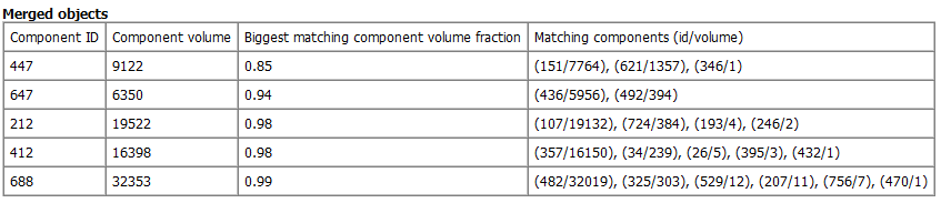

Also the Lost Objects are listed. These are fibers, where parts of them were not detected.

For two-channel cases, the Plots subtab shows the Receiver Operating Characteristic (ROC) curve for each selected structure.

Right-clicking in the plot opens a dialog offering many possibilities to change the plot settings or to save the data. Refer to the Result Viewer handbook to learn more about these options.

When applying a neural network, a confidence field is generated. This field then is segmented with the Threshold given in the Apply Neural Network Options dialog.

Usually, not all voxels are identified correctly. The proportion of voxels correctly assigned to the target material, then is called the True positive rate. The proportion of voxels wrongly assigned to the target material is called the False positive rate.

For a threshold of 0 all solid voxels are assigned to the target material. Thus, the True positive rate and the False positive rate are both 1. For a threshold of 1 no voxels are assigned to the target material and thus, both rates are 0.  

The ROC curve shows how the relation of True positive rate and False positive rate changes if varying the threshold from 0.0 to 1.0.

If the curves look as above, the neural network performs very well on the structures.

The optimum threshold is the upper left area, as the true positive rate is high, but the false positive rate is still low.

The values should lie above of the main diagonal, as otherwise the performance is not better than simply guessing the material IDs. If for all thresholds in (0,1) the true positive rate is 1 and the false positive rate is 0, the network is a perfect classifier, i.e. the result is always perfectly identified materials for all possible thresholds. This means, that the confidence field only contains values near 0 and values near 1, as the neural network is very confident. Usually, obtaining a perfect classifier is not realistic. But it can be close, as in the example above.

The Result Visualization tab provides several 3D visualization options for the results. From the pull-down menu Structure (subfolder) select the subfolder from which the results should be visualized.

If Material Phases was selected for Object Type / Postprocessing in the panel below only the Input structure and the Validation structure showing misclassified voxels are available.

Clicking Load Input Structure (*.gdt) loads the file Input.gdt only containing two material IDs: ID 00 for the background voxels, usually the pore space, and ID 01 for the solid materials.

Click Load Validation Structure (*.gdt) to load the file Validation.gdt.

For two-channel cases, five material IDs are present in this structure and the colors assigned to the material IDs are changed automatically after loading the validation structure:

• ID 00 Pore (invisible): The pore space that is not considered for the identification of target material, in the example it is assigned to air, according to the material IDs in the input structure.
• ID 01 TrueNegative (dark red): the solid voxels that the neural network correctly identified as no target material.
• ID 02 TruePositive (dark blue): the solid voxels that are correctly identified as target material.
• ID 03 FalseNegative (light blue): the solid voxels that are target material, but are not identified as it.
• ID 04 FalsePositive (light red): the solid voxels that are wrongly identified as target material.

These terms come from the confusion matrix commonly used to describe the quality of a neural network.

In the image below, the material phases binder and fibers were distinguished. The voxels correctly identified as fiber (TrueNegative) are visualized in dark red and the correct identified binder in dark blue (TruePositive). The light blue voxels show, where binder was identified as fiber (FalseNegative) and the fibrous voxels identified as binder are marked in light red (FalsePositive). In this example, the neural network identified the binder really well. Only a few voxels at the boundary between fiber and binder were identified wrongly.

For multi-channel cases, each channel gets two material IDs:

• Class # - True Positive: correct identified as class #.
• Class # - False Negative: wrongly not identified as class #.

If Fibers was selected for Object Type, additionally files are available:

• Small fragments which were not assigned to an object
• Fibers which disintegrated into multiple components
• Fibers which merged into a single component.
• Fibers which were not detected

In the following figure, the input fiber structure and the result from FiberFind are shown. The FiberFind result files and result folders can also be found in the Validate Performance result folder.

To check, if there are fragments of solid material not identified as fibers, click Load Fragments (*.gdt) (see the first image below).

Click Load Split Fibers (*.g32) to observe if fibers were split into multiple components (see the second image below).

Also, different fibers can have been merged into one fiber. Click Load Merged Fibers (*.g32) to check on it (see the third image below).

There can be fiber parts not detected as fibers. Click Load Lost Fibers (*.g32) to visualize them (see the last image below).