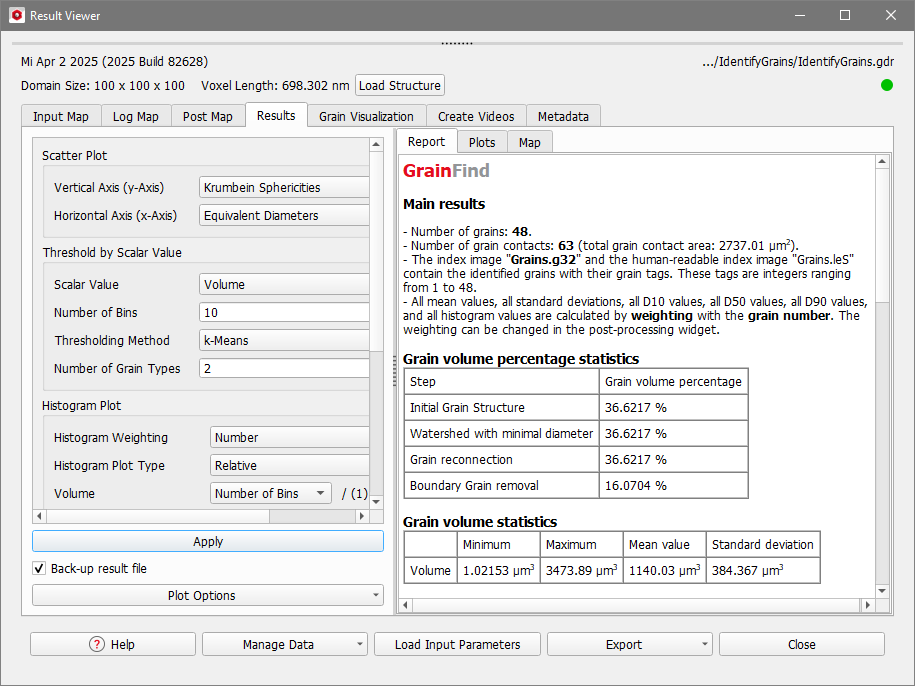
The result file (*.gdr) is opened in the Result Viewer after the computation is finished.
The Results tab is the central point for the analysis of the identified grains. It is grouped in three subtabs: Report, Plots and Map. The Report tab shows statistics about the identified grains and the Plots tab contains plot options for the analysis of the results. The Map tab contains all resulting data from the Identify Grains run. This data is the basis for the tables in the Report tab and for the plots in the Plots tab. On the left, the Post-Processing Widget allows you to fine-tune many graphs of the Plots tab. Collapse the Post-Processing Widget by pulling it to the left.
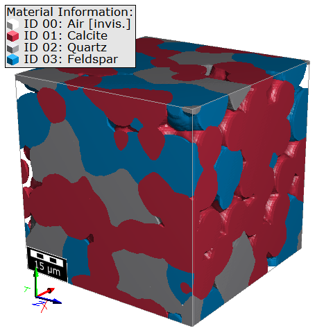
The presented Identify Grains results are computed on this structure with sintered grains, generated with GrainGeo - Sinter. Only Material ID 01 (red) was analyzed.
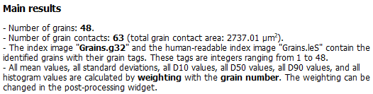
In the Main results section, the number of identified grains and the number of grain contacts is given. For the *.g32 file (and for the *.leS file if Save Grain Index Image as *.leS was checked in the Output Options tab) the range of the index numbers is stated. Below, for the mentioned statistical values, the weighting property is given. This is the same as entered for Histogram Weighting in the Output Options tab, but you can change it later in the Post-Processing Widget.
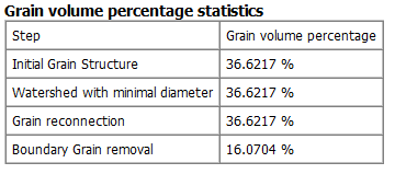
In this table the grain volume during the different steps of the identification are displayed. The grain volume percentage after the Watershed transformation is only shown if Current Structure was chosen as Input Mode. Then, only grains larger than the minimal grain diameter count for the statistics. The volume percentage after Grain-Fragment Reconnection and Boundary Grain removal are only shown if the corresponding options were selected in the options dialog.
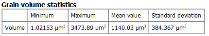
For the identified grains, the minimum, maximum, and mean volume and the standard deviation are shown. The mean value and standard deviation are weighted with the chosen Histogram Weighting (changeable in the Post-Processing Widget).
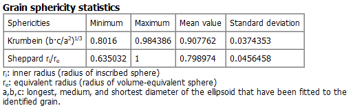
The statistics for the Krumbein sphericity and the Sheppard sphericity (only if Save Inscribed-Sphere Diameters and Sheppard Sphericities was checked in the Output Options tab) are shown. The mean value and standard deviation are weighted with the chosen Histogram Weighting (changeable in the Post-Processing Widget).
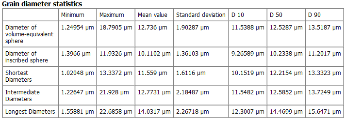
For different grain diameters the minimum, maximum, and mean value and the standard deviation are shown. The mean value and standard deviation are weighted with the chosen Histogram Weighting (changeable in the Post-Processing Widget). Additionally, the characteristic diameters D10, D50, D90 are shown. These are the diameters such that 10%, 50%, or 90% of all grains have smaller diameter than the corresponding value. The Diameter of inscribed sphere is only computed if Save Inscribed-Sphere Diameters and Sheppard Sphericities was checked in the Output Options tab.
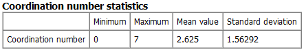
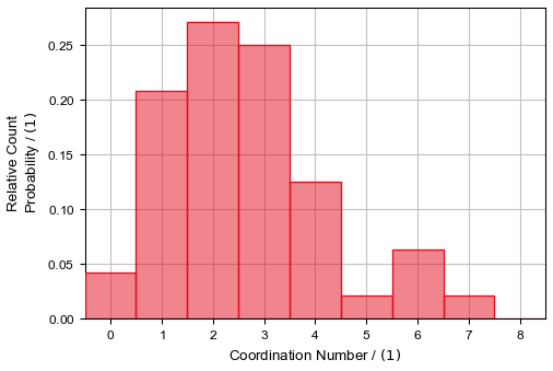
For the coordination number the minimum, maximum, and mean value and the standard deviation are shown. The mean value and standard deviation are weighted with the chosen Histogram Weighting (changeable in the Post-Processing Widget).
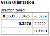
At the bottom, the orientation tensor of all grains is shown.
In detail, let
be the unit vector describing the direction of the k-th object and n the number of objects. Then the orientation tensor T is the sum over the dyadic products of the dk from all n objects, divided by n:
(36) Orientation Tensor
The diagonal elements define the orientation strength for the corresponding directions and sum up to 1. Thus, if for example t11=1 (and t22=t33 =0 ), all objects are oriented in the X-direction. For t11=0 all objects are oriented normally to the X-direction and same values for all diagonal elements (t11=t22=t33= 1/3)) result in a uniform distribution for the object orientation.
Plots
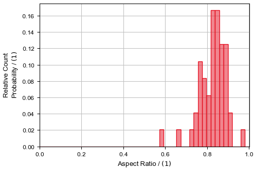
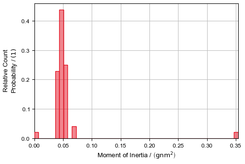
The Plots tab offers several plots to show the relationship between grain parameters: Scatter Plot, Thresholdby scalar value histogram, Volume histogram, Diameters histogram, Perimeter histogram, Sphericities histogram, Aspect ratio histogram, Surfaces And Contacts histogram, Mass histogram, Moment of Inertia histogram, Coordination Number histogram, the Orientation polar plot and the Reconnection Indicators histogram.
Change the plot options in the post-processing widget at the left side of the Plots tab. After changes are made, click Apply… to use the new values. The changes are also applied to the tables under the Report subtab.
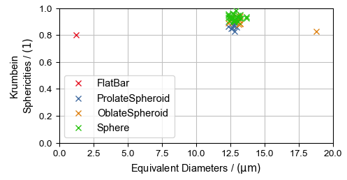
In the Scatter Plot, you can choose two scalar values to be plotted against each other. By default, the Krumbein Sphericity is plotted against the Equivalent Diameters.
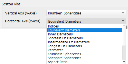
You can change the scalar values in the post-processing widget. The different scalar values are explained in Results of Identify Grains.
The Scatter Plot distinguishes between the four shapes of each object type (Ellipsoids, Short Elliptical Fibers, and Boxes) that are fitted into the grains (see also Pore-Shape Analysis for more information).
In the example above, observe in the Scatter Plot that all identified grains in the structure are nearly spherical (Krumbein Sphericities close to 1). Nearly all grains have an equivalent diameter around 12.5 µm, except of two outliers.
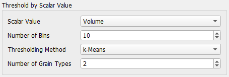
You can classify the grains in the structure into different types based on a chosen scalar value. Define the parameters in the Post-Processing Widget and control the performance in the Threshold by scalar value plot.
First, select the Scalar Value to determine a threshold for from the drop-down list. The default scalar value is Volume. The other scalar values are described under Results of Identify Grains.
The Number of Bins defines how many bins the histogram Threshold by scalar value has. With more bins, a more precise threshold value can be found.
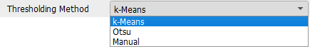
To determine the threshold value, three Thresholding Methods are available:
k-Means: uses the k-Means algorithm to find thresholds for the chosen Number of Grain Types.
Otsu: uses the Otsu algorithm to find thresholds for the chosen Number of Grain Types.
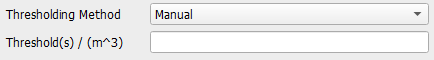
Manual: define your own thresholds by writing a comma-separated list of thresholds into Threshold(s). You implicitly define the number of grain types by the number of thresholds you enter, e.g, if you enter two threshold values this will result in three grain types.
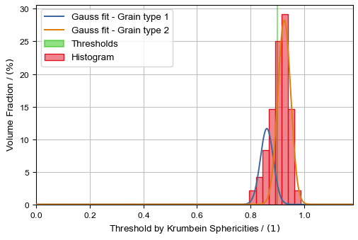
After the settings are made, the Threshold by scalar value plot visualizes the effects. The histogram of the chosen Scalar Value is plotted with the entered Number of Bins. The computed or entered Thresholds are marked as well as the Gauss fit of the grain types. Additionally, a structure containing the different grain types will be created, that can be loaded into GeoDict from the Grain Visualization tab.
In the example, the grains are separated by their sphericity into nearly perfect spheres and more ellipsoidal grains.
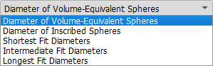
In the Diameters panel you can switch between different plots.
The Diameter of Inscribed Spheres histogram is only available if Save Inscribed-Sphere Diameters and Sheppard Sphericities was checked in the Output Options tab.
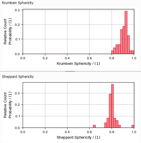
The Krumbein Sphericity and the Sheppard Sphericity (only if Save Inscribed-Sphere Diameters and Sheppard Sphericities was checked in the Output Options tab) are shown in this tab.
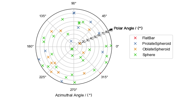
In this tab, the orientation of the fitted grain shapes is plotted as polar plot. This plot distinguishes between the four shapes of each object type (Ellipsoids, Short Elliptical Fibers, and Boxes) that are fitted into the grains (see also Pore-Shape Analysis for more information).
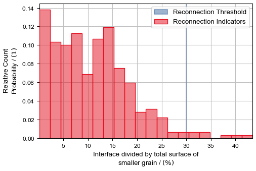
Use the Reconnection Indicators histogram to find an appropriate Reconnection Threshold if you want to use Grain-Fragment Reconnection (find more information in this topic).
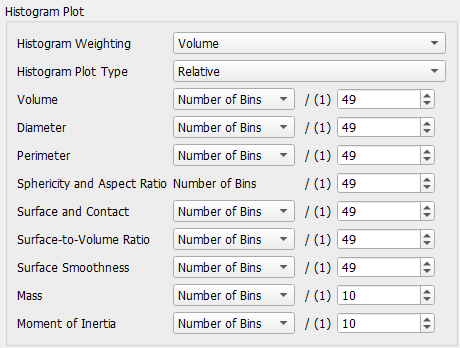
You can modify the histogram plots with the Histogram Plot options in the post-processing widget.
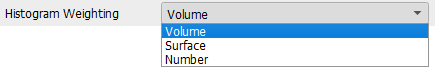
The values on the Y-axes of the histograms in all plots can show Count Probability (weighting by Number), Area Probability (weighting by Surface) or Volume Probability (weighting by Volume), depending on the Histogram Weighting you choose. For the Area Probability (weighting by Surface) the surface area of each segmented grain is computed using the same algorithm as in Estimate Surface Area (MatDict) command and then weighting the grains by that value. The computed surface area does also include the surface between different grains, not only the area between grain and pore material.
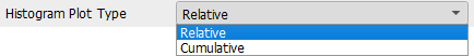
Set the Histogram Plot Type to Relative to compare the individual proportions, or to Cumulative to show the accumulation over the data range.
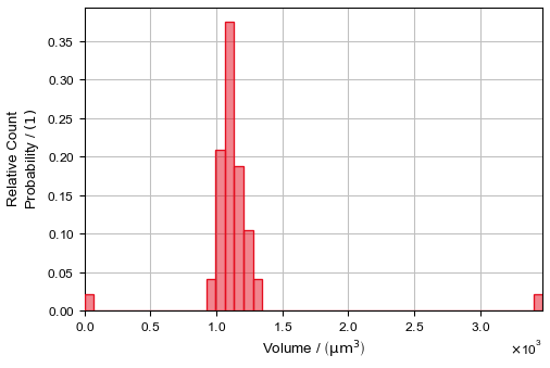
The example on the left-hand side shows, that the smallest grains make up around 20% of the total grain volume. Compared to the weighting with numbers, around 10% of the grains belong to the smallest grains in the structure.
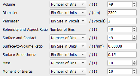
You can customize the bin size for different histogram plots individually. In general, you can choose between:
Number of Bins: choose how many bins the histogram should have.
Bin Size in Units: choose the bin size for the histogram using the value in the displayed unit (e.g. µm, µm3, etc.).
Bin Size in Voxels: choose the bin size for the histogram using the value measure in voxel lengths.
As the different histogram plots show different results, only those choices are available which make sense for the corresponding plot.
The bin size can correspond to one single plot or multiple plots are changed at once:
The selection made under Volume changes the bin size for the plot under the Volume tab.
The selection made under Diameter changes the bin size for all plots under the Diameters tab.
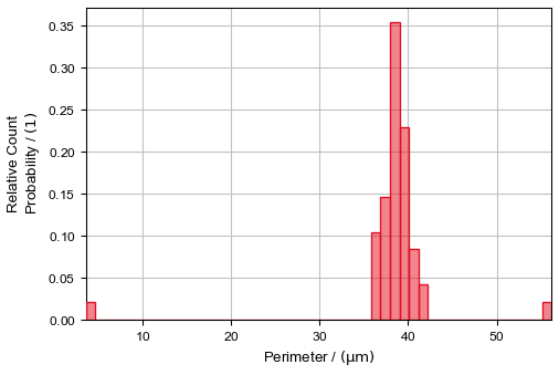
The selection made under Perimeter changes the bin size for the plot under the Perimeter tab.
The selection under Sphericity and Aspect Ratio cannot be changed, this affects the bin size for the plots under the Sphericities tab and the plot under the Aspect Ratio tab.
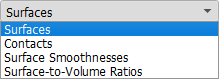
The selection made under Surface and Contact changes the bin size for the Surfaces and Contacts plots under the Surfaces And Contacts tab.
The selection made under Surface-to-Volume Ratio changes the bin size for the Surface-to-Volume Ratios plot under the Surfaces And Contacts tab.
The selection made under Surface Smoothness changes the bin size for the Surface Smoothnesses plot under the Surfaces And Contacts tab.
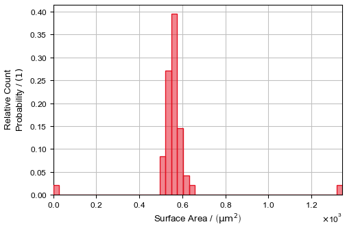
The selection made under Mass changes the bin size for the plot under the Mass tab.
The selection made under Moment of Inertia changes the bin size for the plot under the Moment of Inertia tab.
Post-Processing Widget
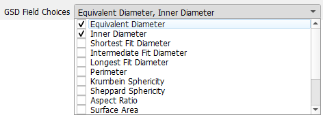
GSD Field Choices
From the drop-down menu choose the scalar grain properties that you want to visualize. For every chosen grain property, a volume field is created containing the 3D distribution of this property. These volume fields are saved together in a *.gsd file (GeoDict size distribution). Load this file in the Grain Visualization tab under Load Grain-Size Distribution.
In the example below, where Equivalent Diameter and Inner Diameter were chosen, the *.gsd file will contain two volume fields: one with the size distribution of the diameters of volume-equivalent spheres, and one with the inner diameter.
 Grain volume percentage statistics