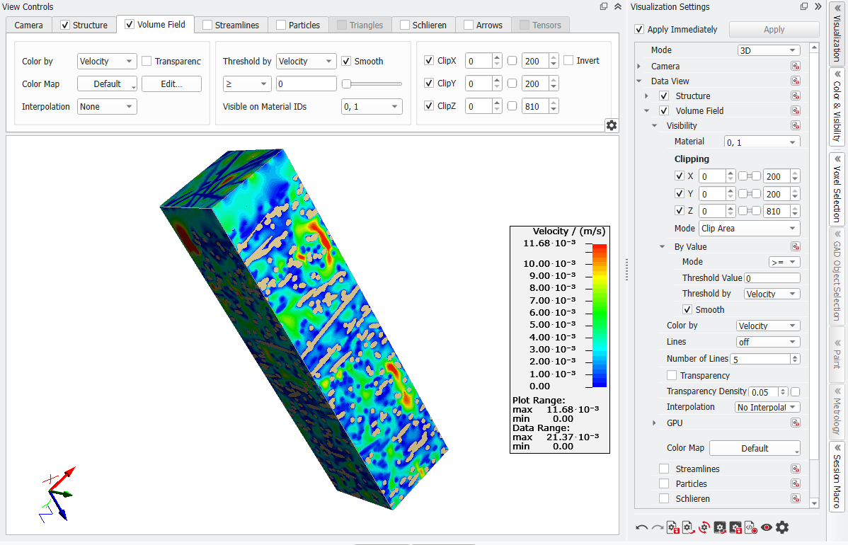
The data of a particular flow field component can be chosen for display from the Color By pull-down menu (here it is Velocity).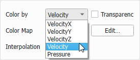

Define different color maps in the Color Map dialog. From the pull-down menu for Color Map in the Visualization tab on the right you can then select between your custom color maps. You can define and select a different color map for each of the components. For example, visualize arrows with the jet color preset and the volume field with the hot preset:

Transparency can be enabled or disabled in the Color Map dialog, from the View Controls or the Visualization Settings dialog. In the Color Map dialog the transparency can individually be set as explained here. In the Visualization Settings dialog, also the overall transparency Density can be changed.

In the View Controls and in the Visualization Settings dialog, several options are available for Interpolation:

• None: For most volume fields, by default, the colors of the volume field are not interpolated and just the raw voxel values are shown.
• Linear: Select to interpolate the colors linearly between surrounding voxel centers.
• Indexed Colors: Only available for integer fields, as for example *.g32 files. For integer fields, usually this is the default setting. If selected, the different index values have distinguishable colors.
• On Visible: Choose to interpolate the colors linearly between surrounding voxels, while not interpolating into invisible areas. Thus, color fringes are removed. In the example below, material ID 01 is selected as invisible. Thus, the flow field is not visualized in the glass fibers. How to choose on which material IDs the volume field is visible is described here.
• On Visible (Smooth): Interpolation works similar to interpolation On Visible, but generates a smooth surface.
• Per Material: Select to linearly interpolate only within the materials to preserve sharp edges.

Below the different interpolation modes are shown for the flow field from the FilterDict simulation:

Below find an example for interpolation on an index field:

The Threshold By pull-down menu in the center panel of the View Controls and, the Volume Field u Visibility u By Value option in the Visualization Settings dialog, allows a clipping that is not related to the spatial coordinates but to the data range. The Threshold By menu has the same options as Color (here VelocityX, VelocityY, VelocityZ, Velocity, and Pressure). You can clip the current fields by values from another field, for example to view the pressure in certain velocities.

Enter the value defining the clipping range below or move the slider. The pull-down menu on the left determines the clipping direction. By default, the threshold mode (or By Value u Mode) displays values greater than or equal to the clipping value, but the user may choose, from the pull-down menu, to display only values smaller than or equal to the clipping value or only values that are equal to the clipping value.

For example, only flow velocities above 0.004 (4 10-03) m/s or then above 0.008 (8 10-03) m/s are visualized.

Observe how the same clipping is done while the pressure field is visualized.

Checking Smooth smoothes the voxel surface of the volume field.

From the pull-down menu Visible on Material IDs select in which material IDs the volume field is visualized. If for example, a flow field is loaded, no flow happens in the solid materials, and thus they can be unchecked.

The displayed data can be spatially clipped in all three directions (ClipX, ClipY, ClipZ) with the sliders or by direct input. This facilitates the simultaneous visualization of, e.g., structure model and flow field. They work as described for the structure clipping.

The settings for the display of flow field isosurface Lines through the Visualization Settings dialog (from the sidebar) are explained for the 2D visualization, and are only visualized, if transparency is disabled.

The GPU section, in the Visualization Settings dialog, offers additional visualization options using the graphics card instead of the main processor, when checking Enabled. The data needs to fit in the GPU memory to use this feature.

Control the amount of Ambient light, Diffuse scattered light and Specular mirror-like highlights, while determining the size of highlights with Shininess. These parameters correspond the Phong Reflection Model, often used in 3D computer graphics. The light intensity controlled by them is independent of the light direction. Higher values for Shininess result in smaller highlights.

Alpha By Grad sets a focus to the edge regions. For high values only the edges are visible.

Alpha By Angle determines the visibility for the current camera angle. Higher values result in a more transparent volume field.

The shading is controlled by the Min Grad (minimal gradient magnitude). Higher values reduce clutter due to noisy data.

The parameters Outline Threshold and Outline Strength apply outlines to the volume field with the given threshold and strength.

With the last parameter determine the overall Density of the volume field.