|
Navigation: GeoDict 2025 - User Guide > Simulation & Prediction > BatteryDict > Battery > Charge Battery > Results |
Scroll |
Results Tab
The Results tab shows the computational results in several ways, through subtabs.
Report
If the solver stopped unexpectedly before one of the stopping criteria defined was reached, the reason for this is shown on top of the report. In the same way, warnings shown before starting the simulation (e.g., due to the parameters selected) and information about the simulation steps for a charging profile are shown there.  |
Afterwards, under Battery, the charge rate applied, the applied current, the charge transferred, and the maximum capacity of the battery cell are listed. The maximum capacity of the battery cell, , is the minimum of the maximum anode capacity, and the cathode capacity, with and denotes hereby the voxel length of the structure, the Faraday constant, and the maximum removable lithium concentration of each active material voxel.  For simulations with the BESTmicro solver, also the produced heat is given in the report. |
 Time dependent charge curve table
The table Time dependent charge curve below shows part of the time dependent values in a clearly arranged way. 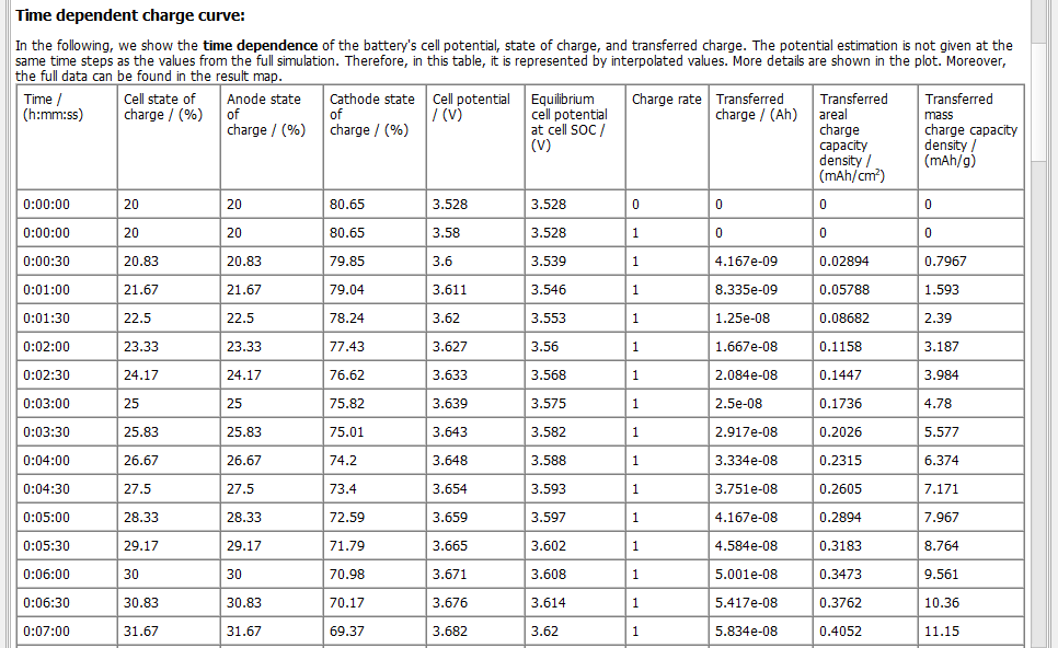 |
For a homogenized simulation with BESTmeso, the Meso parameters computed for both electrodes and the separator are shown below the Time dependent charge curve.  |
Below the Meso parameters or directly below the Time dependent charge curve table the results for the two electrodes are shown respectively, as already shown for the complete Battery above the table, described in more detail above.  |
At the end of the Results-Report subtab for all Charge Battery simulations information about the volumes as already seen in Design Battery or Analyze Battery are found. |
Plots
Under the Results - Plots subtab, several standard plots for the visualization of the BatteryDict simulation results are available. Note that the Lithium concentration and the Potential subtabs of the Plots tab do not exist for simulation results computed with BESTmeso. For the homogenized simulation, the voxel and slice-based information shown on these two tabs is not available.
Clicking the right mouse button allows to change properties of each plot shown, to save the image, or to copy the values to the clipboard. In the same context menu, graphs shown can be switched on and off as well. Find out more details about editing plots in the Result Viewer chapter.  |
On the tab Charge Curves you can select different charge curves from the pull-down menu: Cell potential, Cell state of charge, Cell capacity density, Charge rate, Current density, Current, and Transferred charge are plotted over Time. Additionally, the Cell potential and the Electrode state of charge can be plotted over the Cell state of charge and the Cell potential over the Cell capacity density. 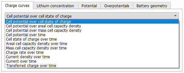 In the Cell potential over Cell state of charge plot the cell potential while charging or discharging is compared to the cell potential in equilibrium, i.e., while loading in infinite time. When the battery is charged or discharged slowly over an infinite amount of time, it remains in a state of equilibrium. However, when the process is done in a finite amount of time, the battery deviates from this equilibrium state. 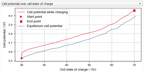 During charging, the curves always show higher values than the equilibrium curve, indicating that charging the battery requires a higher potential than what is observed in equilibrium. On the other hand, during discharging, the curves are always below the equilibrium curve. If Calculate estimation only was chosen as option, the estimation of the cell potential is shown instead of the computed time evolution of the potential. In case a charging profile was selected for the simulation, the cell potential is shown for each simulation step in the profile in a different color. If the charging profile consists of charging and discharging steps, the equilibrium cell potential is shown both for charging and discharging. Start and end point of the whole simulation as well as intermediate start points for the steps are shown in the graph. 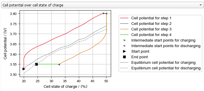 The Cell potential over mass cell capacity density and Cell potential over areal cell capacity density plots show the potential depending on the cell capacity density. The initial cell capacity can be computed from the initial cell SOC and the total cell capacity . The final cell capacity is computed analogously. The transferred charge is the difference between the initial and the final cell capacity. The initial mass cell capacity density can then be computed from the initial cell capacity and the mass of the cell. The final mass cell capacity is again computed analogously. The cell potential over areal cell capacity density takes the SOC value into account. If for example the starting cell SOC is 20%, the starting cell capacity is 20% x Total Cell Capacity (also see equation (166) above. This way, the plot cannot have negative values for charging profiles. For the initial areal cell capacity density follows analogously: For the final areal cell capacity density follows: where NY and NZ are the number of voxels in Y- and Z-direction and VL is the voxel length. The total cell capacity (TotalCapacity) and the transferred charge can be found under the Maps tab in the Battery section. The Mass is given under InputStructure. The domain size and voxel length are given at the top. For our example, the is 70%, the total cell capacity is about 5e-07 Ah, the domain size is 346x300x300 voxel with a voxel length of 400 nm. Thus, for the final areal cell capacity follows: 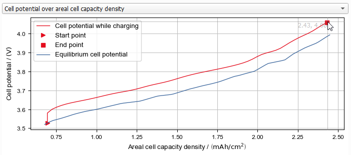 Due to simulation with a constant charge rate in the example shown, the state of charge increases linearly with the simulated time. The trend of the Cell potential over time is therefore the same as for the Cell potential over Cell state of charge and the Cell state of charge over Time is a straight line. The Current over time, as well as the Current density over time, and the Charge rate over time are constant for the example shown. Since GeoDict 2025, the Produced areal heat power over time can also be visualized, when using the BESTmicro solver. During charging and discharging, heat is produced. This causes loss of energy and reduces the charging and discharging efficiency of the battery. Additionally, strong heat production at a single spot can cause a security problem, for example if a polymer separator is melting and a short circuit can occur. This plot displays the areal heat power produced over time. In contrast, a 3D visualization can reveal the specific locations of heat production, helping you determine whether the produced heat is evenly distributed or concentrated in small areas. 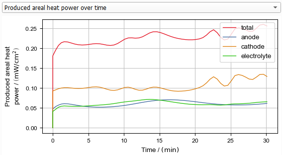 |
The Lithium concentration tab shows the mean concentration of lithium ions for each slice in y-z-direction for a constant x value. It can be displayed as Lithium concentration of electrolyte, Lithium concentration of active material (for all active materials together), or of each active material separately (Lithium Concentration of active material 1, Lithium concentration of active material 2, etc.).  A separate curve is shown in these plots for each state of charge with an intermediate result available. As can be seen in the following plot, the concentration of lithium ions in the cathode (right-part of the plot) is decreasing during charging of the battery, while the concentration in the anode is increasing. 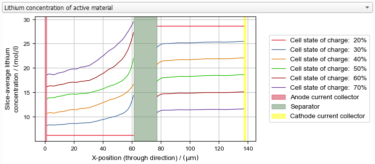 At the beginning of the simulation, the Li-ion concentration of the electrochemically connected part of the electrolyte is constant throughout the battery. Its value is the equilibrium Lithium concentration specified in the settings. While charging, the cathode releases Li-ions into the electrolyte, causing the Li-ion concentration to increase on the cathode side. Simultaneously, the Li-ions intercalate into the anode. Since the diffusion of the Li-ions takes some time, the gradient of the Li-ion concentration in the electrolyte is visible in the example. 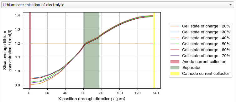 |
The Potential tab shows the mean potential for each slice in y- and z-direction for the solid part of the battery, as well as for the electrolyte. All potentials are calculated with respect to an imagined lithium reference electrode in the center of the separator. Again, for each state of charge with an intermediate result available, a separate curve is shown in the plot. Click the right mouse button in the plot to change view settings as shown in the Result Viewer chapter. 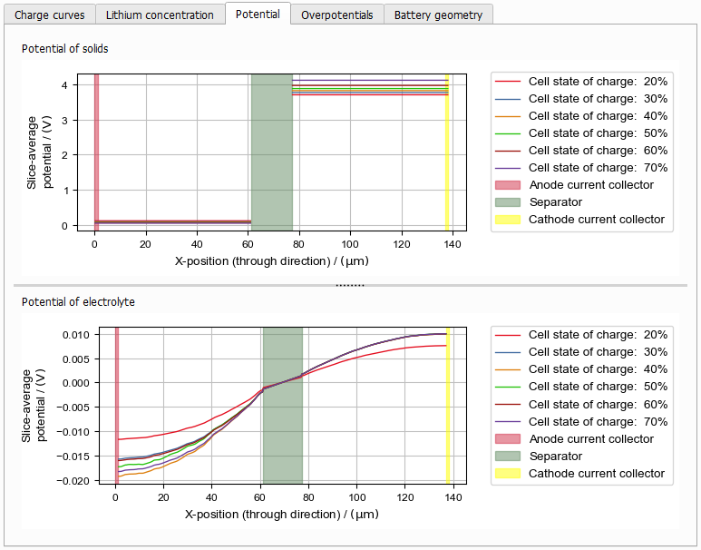 In the example shown here, for each time step, the potential in the solid is constant within each electrode. This indicates that the conductivity is high enough. If the conductivity were much smaller, the potential would exhibit a drop within one electrode. In this example, the solver calculates the battery charging by applying a constant electric current. The necessary potential difference for keeping up the current is determined from the electric current in the solids, the ionic current in the electrolyte, and the overpotentials on the boundary of electrolyte and active material. The current is only dependent on the potential difference and not on the total potential offset. The latter can be chosen freely. For the potential of the electrolyte, a gradient is visible between the anode current collector and the cathode current collector. This gradient increases for higher charge rates and the potential grows from left to right. This is caused by the charge current that is driven by the ions resolved in the electrolyte. The charge current leads to a growing potential in flow direction because the ionic conductivity is not zero. The lower the ionic conductivity, the stronger the growth of the electrolyte potential in flow direction. |
On the Overpotentials tab, the evolution of the different overpotentials over time is visualized. For an explanation of the overpotentials also see here.  # # |
The Battery geometry tab shows the mean of porosity and the volume fraction of active material for each slice in y- and z-direction.  |
Map
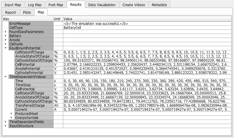
The Results - Map subtab lists all values available in the Results - Report subtab of the Result Viewer of the GeoDict result file and other information about the computation results.
©2025 created by Math2Market GmbH / Imprint / Privacy Policy
