The Watershed Transformation treats the image it operates on as if it were a topographic map. In this model, the brightness of each pixel represents its elevation. The computation then finds lines running along ridge lines. The Watershed (Supervoxel) is based on the Euclidean Distance Transform (EDT). Seeds for the Watershed component are placed at the local maxima of the EDT. In these seeds, components begin to grow. During this growth process, component boundaries form as soon as components touch.

The implemented algorithm detects edges in the imported image based on the gray value or morphological gradient (see Preprocessing). Then, a distance map is created based on the edge distances. The maxima in the distance map (see the image below) are used as seeds for the watershed algorithm, which is then performed on the distance map.

The concept of a watershed is easier to understand with a 2D example. In this representation, the EDT is a topographical relief where high values represent valleys and low values represent peaks. This topography is continuously flooded with water, beginning with the deepest valleys. As soon as water from a neighboring valley begins to mix in, a dam is created, corresponding to a material boundary. The result is a topography with water-filled valleys separated by dams. The identified valleys represent watershed components, and the dams separating them denote component boundaries.

The figure below illustrates the progression of the watershed algorithm. On the left, the topographical relief corresponding to the EDT is shown, with the component seeds (valley bottoms) marked in red. This topography is successively flooded with water, forming dams between adjacent valleys. Information about the component space, such as the minimum component diameter, can be used to adjust the Watershed (Supervoxel) results. Each watershed component is assigned the mean gray value of that component. This is the supervoxel. The result is a gray value image that is much easier to segment.

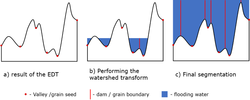
If there are artifacts in the initial image, it is recommended to apply other image filters, such as the Non-Local Means Filter, before running the Watershed (Supervoxel) algorithm. This will lead to better results.

The name for the file and folder containing the results can be entered in the Result File Name (*.gdr) box. Choose a name fitting the current project.

Preprocessing

Seeding

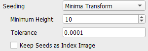
Click Apply to run the watershed algorithm.

Results

The result file with the specified Result File Name is opens automatically in the Result Viewer. The number of watershed components and their minimum, maximum, and mean sizes can be found under the Results – Report sub-tab.

Go to the Data Visualization tab and click Load *.g32 to visualize the Index Image of Watershed Components in the GeoDict visualization area. This image shows the individual regions identified by the watershed. For the filtered image visualized in the Image Processing dialog, the resulting gray value is the mean gray value of the corresponding region. If the watershed identifies individual objects, the components file can be used as input for GrainFind Identify Grains, for example. However, for many scans, the individual objects cannot be recognized from the gray value image.

If the Keep Seeds as Index Image box is checked, the watershed seeds can be visualized by clicking the lower Load *.g32 button. Otherwise, the button is grayed out. This image shows the seeds specified by the H-Minima Transform algorithm. Use it to rerun the watershed with different preprocessing parameters, as explained above. In the opening dialog, click OK to load the index image in GeoDict. For more information about GeoDict result files, refer to the Result Viewer user guide.

Example

In the following example, a Morphological Gradient with Gradient Radius 2 was applied ,and for the Minima Transform a Minimum Height of 15 was used. Note the difference in the resulting Histogram, which makes it possible to simply apply the automatic Otsu threshold.