In the Scatter Plot panel, you can choose two scalar values to be plotted against each other. By default, the Krumbein Sphericity is plotted against the Equivalent Diameters.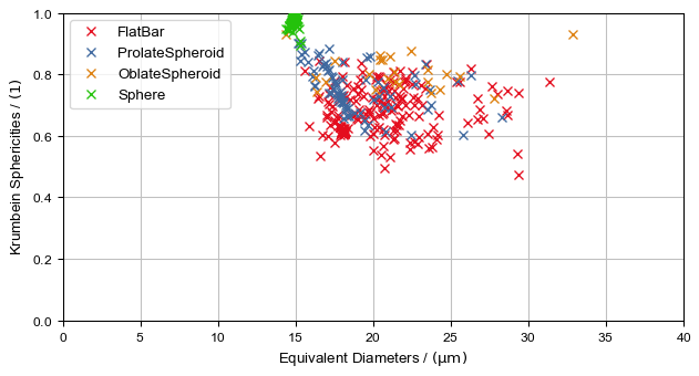

You can change the scalar values in the post-processing widget. The different scalar values are explained in Results of Identify Pores.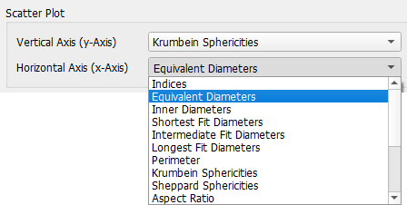

The Scatter Plot distinguishes between the four shapes Flat Bar, Prolate Spheroid, Oblate Spheroid, and Sphere. These are the four possible shapes for the ellipsoids that are fitted into the pores (see also Results of Identify Pores for more information). In the example above, observe in the Scatter Plot that the found spherical pores have an equivalent diameter of 15 µm, while the other found ellipsoids have equivalent diameters between 15 and 32 µm.

You can classify the pores in the structure into different types based on a chosen scalar value. Define the parameters in the Post-Processing Widget and control the performance in the Threshold by scalar value plot.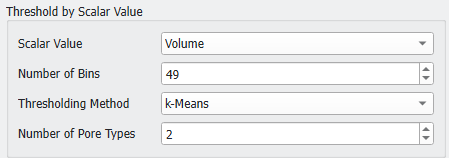

First, select the Scalar Value from the drop-down list to determine a threshold for. The default scalar value is Volume. All scalar values are described under Results of Identify Pores.

The Number of Bins defines how many bins the histogram Threshold by scalar value has. With more bins, a more precise threshold value can be found.

To determine the threshold value, three Thresholding Methods are available:

• k-Means: uses the k-Means algorithm to find thresholds for the chosen Number of Pore Types.

• Otsu: uses the Otsu algorithm to find thresholds for the chosen Number of Pore Types.
• Manual: define your own thresholds by writing a comma-separated list of thresholds into Threshold(s). You implicitly define the number of pore types by the number of thresholds you enter, e.g, if you enter two threshold values this will result in three pore types.

After the settings are applied, the Threshold by scalar value plot visualizes the effects. The histogram of the chosen Scalar Value is plotted with the entered Number of Bins. The computed or entered Thresholds are marked as well as the Gauss fit of the pore types. Additionally, a structure containing the different pore types will be created, that can be loaded into GeoDict from the Pore Visualization tab.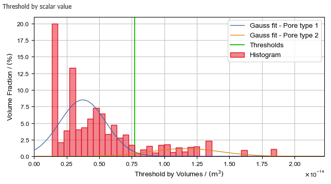

In this tab the Volume of the identified pores is plotted. The Histogram Plot Options are explained below.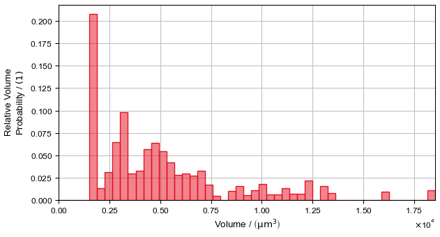

In the Diameters panel you can switch between different plots.

The Diameter of Inscribed Spheres histogram is only available if Save Inscribed-Sphere Diameters and Sheppard Sphericities was checked in the Output Options tab.

The Histogram Plot Options are explained below.

In this tab the Perimeter of the identified pores is plotted. The Histogram Plot Options are explained below.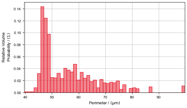

The Krumbein Sphericity and the Sheppard Sphericity (only if Save Inscribed-Sphere Diameters and Sheppard Sphericities was checked in the Output Options tab) are shown in this tab.

The Histogram Plot Options are explained below.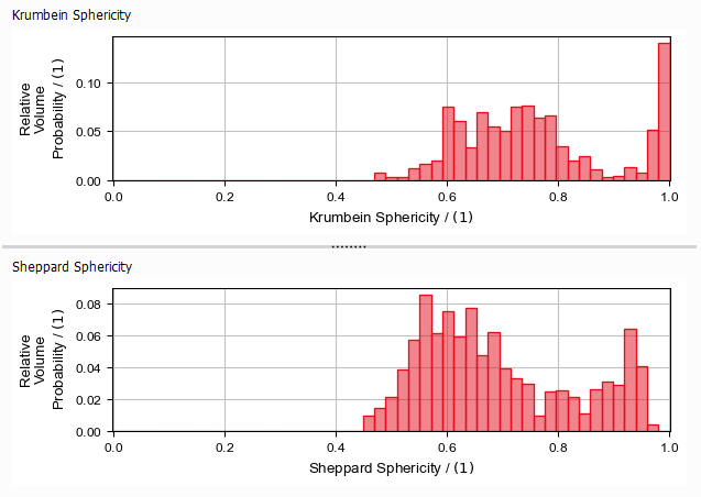

In this tab the Aspect Ratio of the identified pores is plotted. The Histogram Plot Options are explained below.

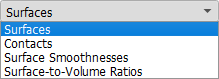
In the Surfaces and Contacts panel you can switch between different plots.

The Histogram Plot Options are explained below.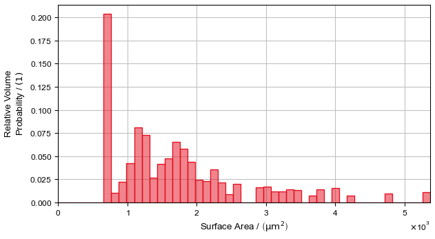

In this tab the Coordination Number of the identified pores is plotted. The Histogram Plot Options are explained below.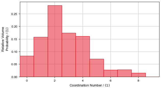

In this tab, the orientation of the fitted pore shapes is plotted as polar plot. This plot distinguishes between the four shapes Flat Bar, Prolate Spheroid, Oblate Spheroid, and Sphere. These are the four possible shapes for the ellipsoids that are fitted into the pores (see also Results of Identify Pores for more information).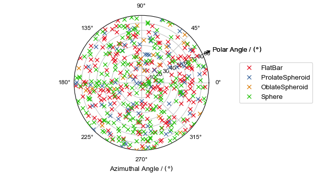

Use the Reconnection Indicators histogram to find an appropriate Reconnection Threshold if you want to use Pore-Fragment Reconnection (find more information in this topic).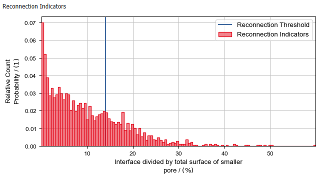

You can modify the histogram plots with the Histogram Plot options in the post-processing widget.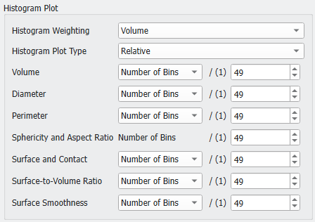

The values on the Y-axes of the histograms in all plots can show Count Probability (weighting by Number), Area Probability (weighting by Surface), or Volume Probability (weighting by Volume), depending on the Histogram Weighting you choose. For the Area Probability (weighting by Surface) the surface area of each segmented pore is computed using the same algorithm as in Estimate Surface Area (MatDict) command and then weighting the pores by that value. The computed surface area does also include the surface between different pores, not only the area between pore and solid material.

Set the Histogram Plot Type to Relative to compare the individual proportions, or to Cumulative to show the accumulation over the data range.

The example on the left-hand side shows, that the smallest pores make up around 20% of the total pore volume. Compared to the weighting with numbers, 42% of the pores belong to the smallest pores in the structure.

You can customize the bin size for different histogram plots individually. In general, you can choose between:

• Number of Bins: choose how many bins the histogram should have.
• Bin Size in Units: choose the bin size for the histogram using the value in the displayed unit (e.g. µm, µm3, etc.).
• Bin Size in Voxels: choose the bin size for the histogram using the value measure in voxel lengths.

As the different histogram plots show different results, only those choices are available which make sense for the corresponding plot.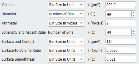

The bin size can correspond to one single plot or multiple plots are changed at once:

• The selection made under Volume changes the bin size for the plot under the Volume tab.
• The selection made under Diameter changes the bin size for all plots under the Diameters tab.
• The selection made under Perimeter changes the bin size for the plot under the Perimeter tab.
• The selection under Sphericity and Aspect Ratio cannot be changed, this affects the bin size for the plots under the Sphericities tab and the plot under the Aspect Ratio tab.
• The selection made under Surface and Contact changes the bin size for the Surfaces and Contacts plots under the Surfaces And Contacts tab.
• The selection made under Surface-to-Volume Ratio changes the bin size for the Surface-to-Volume Ratios plot under the Surfaces And Contacts tab.
• The selection made under Surface Smoothness changes the bin size for the Surface Smoothnesses plot under the Surfaces And Contacts tab.