|
Navigation: GeoDict 2025 - User Guide > Image Analysis > GeoDict-AI > Train Neural Network |
Scroll |
AI Options
Under the AI options set-up the training of the neural network.
Input Data
In the Input Data panel specify the training data.
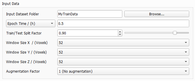
Browse for the Input Dataset Folder containing the subfolders Train and Test. This folder is filled with training data when running Create Training Data or manually. |
 Epoch Time and Downsampling Factor
Define the duration of one epoch, either directly by selecting Epoch Time or by selecting Downsampling Factor. This defines how often an intermediate neural network is saved to the result folder. Also, considering every possible window position in the structure as described for Window Size leads to a large amount of data. The amount of data is reduced by the given epoch time or the downsampling factor. For Epoch Time enter a time, usually between 0.1 and 0.5 hours. Then, the entered value will be the exact time of the first epoch to find out the needed number of samples (or window positions). All following epochs will use the same number of samples, such that all epochs will need approximately the same time. The maximum number of epochs can be entered under the Stopping Criterion tab. The Downsampling Factor is a value in [0,1] which is used to directly reduce the data amount during training. After loading all the data defined by the window size, GeoDict-AI will ignore some of the data samples depending on the factor, e.g., if 0.1 is specified, a random 10% subset of the data will be retained. The data is sampled uniformly from all structures. For the training in most cases a downsampling factor between 0.01 or 0.001 is recommended. However, this depends on the amount of training data. The larger the amount of training data, the smaller the Downsampling Factor should be chosen for a higher frequency of intermediate results. The larger the downsampling factor, the longer the runtime of one epoch. But for a larger factor, less epochs are needed to reach the same result. This means, while the downsampling factor affects the training time of one epoch, it does not significantly affect the overall training time.
|


Before starting with the training, the training structures (images) - generated with Create Training Data or manually - are split into all the windows defined by Window Size. After permuting these windows randomly, the Train/Test Split Factor determines the number of windows which are used for the training and how many are used for the evaluation during training. This way, the structures (images) from the Train folder are divided in train and test data and all training structures are represented in the train data as well as in the test data. The default value 0.9 means that 90% of the windows are used for training and 10% for evaluation. The 10% of the training data are used for internal tests during the training, i.e. to compute the validation loss by applying the neural network to these structures (images) at the end of each epoch. This is necessary to have a measure on how well the network can generalize what it has learned to the new data. In most cases, the default of 0.9 for the split factor produces good results.
|
The Window Size determines the size (in X, Y and Z) of the sampling window in voxels. The training data consists of several input and output files. For the training cutouts from corresponding input and output files are taken in the same location with the given window size. Thus, all network’s decisions are based on these cropped data pairs alone. The neural network will try and learn to transform what it sees in the input window to what it observes in the output window. The Window Size determines how much context the network obtains for its decisions. Larger values improve the performance, while increasing training time and GPU (memory usage). Any possible placement of the window within the structure corresponds to a potential training sample. However, considering all possible locations during one epoch is usually redundant and prohibitively expensive in terms of runtime. To reduce this large amount of data, the parameters Downsampling Factor or Epoch Time are used. The Window Size must be large enough to capture an entire important feature, e.g. a fiber crossing with binder. This way it is possible to distinguish the different materials only from the window. For a fiber structure, for example, it is recommended to choose the window bigger than twice as large as the diameter of the largest fiber. This allows two touching fibers to be fully contained in a single window. This way the network can correctly identify the geometric configuration, as two fibers crossing or touching and hence, make an informed decision about the binder placement around the touching point. Consider differentiating binder and fibers only based on a cutout in the selected window size. If a human cannot distinguish the material phase from the geometry seen in the cutout window, it is unlikely that a neural network is capable to. In such cases, the window size must be increased so the neural network can "see" the two fibers approaching each other and trace them through the intersection even with the large amount of binder obscuring the actual intersection point. If it is humanly possible to identify the binder, the network can also learn that. Otherwise, the window size must be increased. In the next figure, different window sizes are considered. Observe how in a) it is easy to distinguish binder from fibers, as the window size is larger than twice the fiber diameter. In image b) it is already hard, but still possible with a window size only a little more than twice the fiber diameter. However, in a cutout even smaller than twice the fiber diameter as in c) it will be nearly impossible to identify the fibers.  The aspect ratio of the window can be adjusted to the corresponding structure, e.g. for a flat textile structure or for materials which are anisotropic. For example, in the gas-diffusion-layer of a fuel-cell the fibers are usually oriented mainly in the X/Y-plane. Then, a smaller window size in Z-direction is reasonable. For isotropic materials, however, it is recommended to set the window size for all three directions to the same value. The possible values for Window Size also depend on the Depth selected for the UNet model. In each convolution 1 voxel is lost at each border of the cutout. As there are two convolutions in each layer of the UNet, four voxels are subtracted from the window size in each direction (compare to the UNet diagram. The resulting values are divided by two in each max-pool operation. The selected Depth determines the number of applied max-pool operations. Select the Window Size from the pull-down menu. When changing the Depth or the Size of Convolutional Kernel in the UNet dialog, the pull-down menu for window size is automatically updated and the smallest available window size is selected. In the following table find possible window sizes for reasonable depth values (and a kernel size of 3). While the pull-down menus also offer larger values, in most cases a window size larger than 200 will not be possible with the given hardware.
|
The Augmentation Factor allows to effectively increase the amount of training data. For the default of 1 (No Augmentation), each window is seen once during a training epoch. Setting it to 48 (Full data augmentation, all rotations), the window will also be mirrored and rotated, effectively increasing the data set size by factor 48 with the corresponding increase in runtime. The option of factor 16 (No rotations out of the XY plane, for anisotropic geometries) which is specifically for structures where fibers are mainly oriented in the XY-plane. Then, only mirroring and rotation in the XY-Plane is performed. However, values higher than 1 are mostly useful for a small data set, e.g., a single structure, to get as much information as possible from it. |
Neural Network
In the Neural Network panel define the parameters for the network.
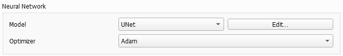
The pull-down menu for Model contains the neural network architecture that is being used for training. Currently only the UNet is available, which performs very well for segmentation tasks. In future releases, more models will be added. Clicking Edit opens the Set Model Parameters dialog. In this dialog the reference Ronneberger, Fischer and Brox, 2015 describes the underlying architecture of the UNet. Increasing the parameters Depth of the UNet and Number of Features in First Layer improves the performance of the network, but also significantly increases the training time and the amount of used GPU memory. 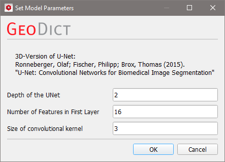 The UNet has a U-shape (hence the name) with a constricting and an expanding branch on the left and right respectively. The diagram below shows a UNet with depth 2, 16 features in the first layer and a window size of 52 voxels in X-, Y- and Z-direction. Find a detailed description of the diagram here. The Depth of the UNet corresponds to the number of layers in each of the branches. Increasing the depth massively increases the complexity of the network, but also the amount of abstraction that it can perform. In Ronneberger, Fischer and Brox, 2015 the UNet operates in 2D, allowing the authors to use a depth of 4, but since GeoDict-AI performs 3D analysis the limits of GPU memory are reached quickly when increasing this parameter. In general, only 2 or 3 are possible and it is recommended to use the default of 2. In the diagram the depth is the numbers of Max Pool or Deconvolution operations. The Number of Features in the First Layer corresponds to the last shape specification coordinate in the diagram in the first layer on the left, and it determines how many different types of features (edges, corners, blobs...) the network will learn to detect in the first layer. In the diagram, after the first convolution, 16 features are considered. Thus, the number of features in the first layer is 16. In most cases the default of 16, which is the minimal value, delivers good results for testing the training settings. Once it is ensured, the trained network performs well, larger values can be used for further improving the performance. The subsequent layers in the contracting branch will double the number of features in every step. This is a standard construction for these types of networks. In the contracting branch the image resolution is reduced while the information depth (number of features) is increased. Thus, increasing the parameter also increases the amount of GPU memory required. Control the Size of the Convolutional Kernel. A kernel is a feature detector, i.e. a n x n x n voxels box with a defined pattern as described here. The size n is the number of voxels in one direction and must be an odd number. Common values are 3 or 5. |
For the Optimizer select between Adam and SGD. The optimization algorithm iteratively updates the network weights according to the current training data. For many applications, the Adam optimizer leads to faster convergence, but the SGD (stochastic gradient descent) optimizer can result in a slightly better result. In most cases using Adam is recommended. If all other parameters work well to the current training, but the result is not already perfect, run a final production training run with SGD. For theory about Adam refer to Kingma and Ba, 2016, and for more information about the SGD method see Ruder, 2016. |
Description Text
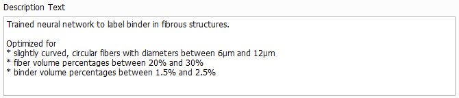
The Description Text can be edited as desired and will be displayed in the Apply Neural Network dialog when loading the trained network. It should contain the purpose of the model and the assumptions made during training, e.g. the fiber diameter range and the solid volume percentage range. Thus, the user applying the model can decide if the model applies to their structure.
|
Important! The description cannot be changed after the training. Thus, always remember to enter a meaningful description before starting the training. |

©2025 created by Math2Market GmbH / Imprint / Privacy Policy