AI Segmentation
The AI Segmentation allows you to train machine learning algorithms to segment the complete gray value image based on user-defined labels. To accomplish this goal, label the image manually and train a machine learning method that learns how to segment the image based on the provided labels.
The name of the file and folder containing the results can be entered in the Result File Name (*.gdr) box. Choose a name fitting the current project.
The four different AI Models Boosted Tree, Random Forest, Unet2D, and Unet3D are described in this chapter. In the following table, the learning methods are compared directly.
Random Forest and Boosted Tree Since GeoDict 2023, the AI-segmentation via the widely used Random Forest method is featured in addition to the Boosted Tree method. Both methods work very similar, but the Boosted Tree model is usually faster, since it is an advanced version of the Random Forest. Boosted Tree and Random Forest both work well for many examples and are very fast. For the training data, information about the neighboring voxel data are used and different filters are applied to the input image:
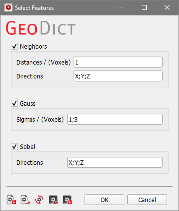
Define the filter parameters for these images and to which distance the neighboring voxels should be considered in the Select Features dialog explained below or simply use the default values. In the figure below, three filtered images are used, one with a small sigma for the Gauss filter, one with a larger sigma, and one image filtered with the Sobel filter. Then, for each voxel a vector is built containing the corresponding data from the original image, from each of the filtered images, from the neighboring voxels, and from the labeled image. In the diagram below this is shown for two voxels. The Random Forest / Boosted Tree algorithm learns from these vectors and segments the image. 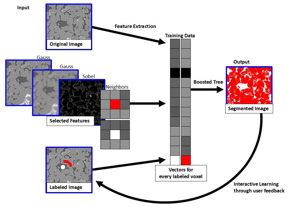
In the case of big-scaled relevant features, the Random Forest and Boosted Tree methods can be limited. That is because the decision for each pixel depends on the surroundings, especially on the Gauss kernel of a fixed size. If, e.g., the image has pores of different materials but with a similar gray value and the only difference is the border to the solid material, for big pores the boosted tree method could decide wrong. In such cases, the Unet methods are recommended. Also, if more than two materials are in the structure, they can be limited and the Unet method is preferable. Click on the gearwheel icon
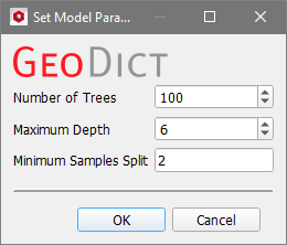
 The following parameters can be set for the Random Forest model:
 For Boosted Tree and Random Forest the Select Features dialog controls the parameters for the applied filters for the Boosted Tree and the Random Forest methods. 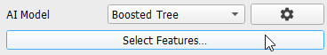 These filtered images are considered in the training of the model as shown in the figure above to gain more information for each voxel. They are used also in the segmentation, but only as a reference for the model, since they can help to identify which label is correct for which voxel in the original image. These filters always were applied for Boosted Tree with the current default settings, but since GeoDict 2023, their parameters can be changed by you. Check the features that should be used and enter a list of parameters for the feature runs, separated by “;”:
 Unet The deep learning methods Unet2D and Unet3D require more training data. Thus, more labels must be provided manually. However, they are more capable to analyze the scan correctly and thus, achieve better results. The name Unet refers to the U-shape of the neural network diagram, consisting of a constricting branch on the left and an expanding branch on the right. The number of layers in each branch defines the depth of the Unet. 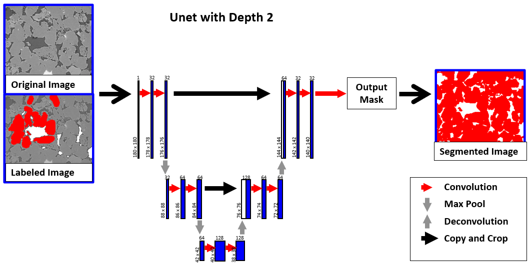
To use the Unet models a good graphics card is needed, i.e., a NVIDIA graphics card (GPU) with compute capability of at least 3.5. Make sure that the drivers are installed and up-to-date. See more information on graphics cards at https://developer.nvidia.com/cuda-gpus. This webpage contains a helpful section with Frequently Asked Questions. For Linux, the Gnu C Library (glibc) must be at least version 2.17. We recommend Ubuntu 20.04 LTS, but for a current glibc other Linux distributions should also work. Unet3D considers the complete image, while Unet2D learns from a single slice in the specified direction. The default is the Z-direction. Click on the gearwheel icon
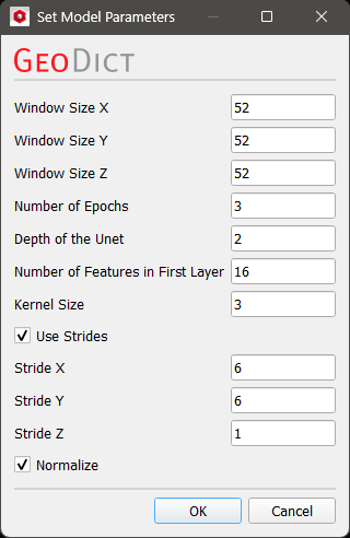 For a more detailed explanation about the Unet parameters refer to the GeoDict-AI user guide. Unet2D means that the windows determined by Window Size are 2D slices, i.e., one of the three Window Size parameters is 1. The default for Window Size Z = 1 usually leads to good results. If all three size parameters are greater than 1, the Unet3D model is applied automatically. The choice of Batch Size is only available for the Unet models and is the number of samples the training uses simultaneously. For example, with a batch size of 4, during training the error is computed, and the network updated for one window at the same time, before moving on to the next four windows. In literature there is usually a warning about too large values for batch size due to the potential of overfitting. However, in 3D image analysis the batch size is limited by the available GPU memory. If the value is chosen too high, a warning dialog appears, when starting the training. It is recommended to set the value as high as possible with the available GPU memory, so that the training works without giving an error. This is often a value between 1 and 8 depending on the GPU hardware. Modern GPUs can allow for even higher values for the batch size. If multiple GPUs are available, select on which it should run, by checking the corresponding checkboxes. If licensed, multiple GPUs can be used for the training and segmentation. Then, the batches are distributed to equal numbers on the different GPUs. If no GPU is detected, the training and the AI-segmentation are run on the CPU, which usually needs much more runtime. 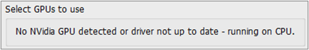 The Select Additional Images dialog controls which of the loaded images should be considered for the training additionally to the current image. Multiple images can be loaded to the Image Processing dialog by having Keep existing Volume Fields selected in the Import Geometry dialog. Thus, it is possible to take multiple images from the same structure’s cutout into account for training. For this, the images must be the same size and fit to the used labels. If the network was trained on several images, these images also are needed for the segmentation. Different scanning settings can produce different kinds of images. For example, if an image has three material phases it can sometimes be hard to get a good contrast for all three of them at the same time. Then, the image can be taken twice, once with a good background separation and once with a good contrast between the solid materials. For the training the neural network considers both data sets and thus, will generate better results, compared to only considering one of these images. 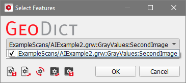 |

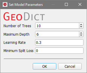
 gives access to the parameters defining the model setup. The Set Model Parameters dialog opens. The following parameters can be set for the Boosted Tree model:
For all models, choose the Number of Materials to be labeled in the scan. 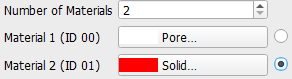 Specify the different materials with the material database. The checkbox next to the material boxes determines the current material for painting the labels. The Navigation Mode Select the Painting Mode Make sure to have approximately the same amount of labeled area for the different materials, especially for the Unet models. Validate this in the Label Data tab of the Histogram section. If a label was not painted correctly switch to the Erasing Mode Change the Brush Size fitting to the areas to label. When you enable the Magic Brush the images are analyzed on clusters recognizing edges. The Magic Brush clusters are computed using the SLIC (Simple Linear Iterative Clustering) algorithm, which generates the cluster based on gray value similarity and proximity in the image plane. Then, labels can be created by simply left-clicking on these clusters in Painting Mode. To show the clusters, enable Show Magic Brush Outlines. You can change the size of the created clusters by changing the Brush Size. For many image datasets this feature makes labeling much easier. 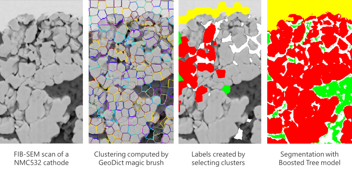 Using the different view directions, you can observe the already existing labels from slices labeled in the other two directions, respectively. In the example below, the center slices in X- and Z-direction were labeled. Thus, if viewed in Y-direction, two thin lines with white (material 1) and red (material 2) sections are already labeled. If labels are erased on these lines, in the respective slices in the other directions thin lines are erased. This leads to less training data. 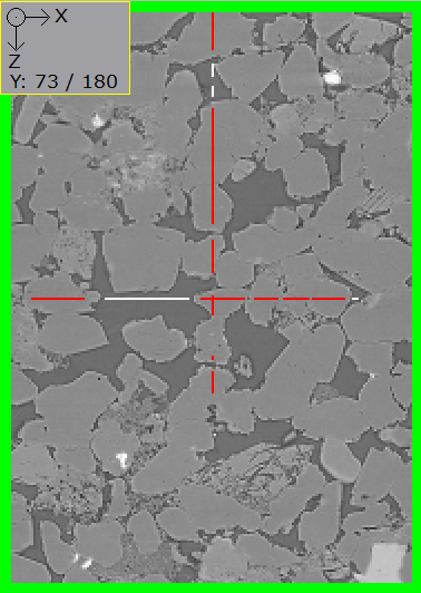 If there are more than two materials, it is important to label boundaries for all different boundary combinations. Labels close to each other give better results. For each labeled area paint as many labels as possible to get a fully filled output window. While it can be important to label boundaries, only label as near to the boundary as it can be ensured to label it correctly. Otherwise, wrong training data will be generated. Paint in all three directions, especially if the gray values differ much. Especially for the Unet3D method ensure to label some consecutive slices in the same areas. Save the painted labels as *.gld file by clicking Save Labels. Load the training data again whenever needed by clicking Load Labels. Delete all labels by clicking Clear Labels.  If a trained model is loaded, the Overlay can also be set to Preview to preview the segmentation results for the current slices. When changing the Overlay to Mixed, both the current Labels and the Preview of the current model can be viewed. If the preview shows that the model needs more training, using the mixed view helps to concentrate the further labeling on the areas, where the model did not classify the voxels correctly. |
 allows to pan the image in the 2D Slice Visualization section with the left mouse button and zoom in and out with the right mouse button.
 to paint in the 2D Slice Visualization area. Ensure to have the Visibility turned on as described
  and erase labels by clicking or holding the left mouse button and moving the mouse over the labels.
 Train and Apply a Neural Network
After clicking Create Segmentation for one of the segmentation methods, the segmentation is applied for the gray value image. For Global Thresholding, AI Segmentation, Multi-Phase Segmentation, and Hysteresis Thresholding a result file (*.gdr) is generated and saved in the project folder. The generated result file with the name entered for Result File Name is opened automatically in the Result Viewer. The Report tab lists some basic Structure Information for the resulting structure and all steps done in the Image Processing dialog, e.g., Segmentation methods and the used Image Filters. In addition to the result file, a result folder with the same name is saved inside the current project folder, containing the segmented structure file (*.gdt) and, for the AI segmentation, also the used labels (*.gld), and the trained model (*.FOREST, *.XGBM, *.UNET2D or *.UNET3D). For a more detailed description of the Result Viewer options refer to the Result Viewer user guide. 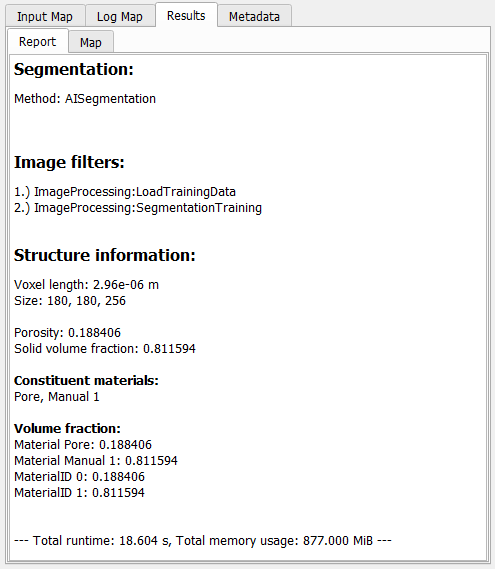 |
©2025 created by Math2Market GmbH / Imprint / Privacy Policy